Unemployment: autoregression and posterior predictive checks

Source: Unemployment/unemployment.Rmd

The original fits a first-order autoregression and checks whether simulated unemployment series reproduce the observed sign-change behavior.

Code

from pathlib import Path
import numpy as np
import pandas as pd
import matplotlib.pyplot as plt
import statsmodels.formula.api as smf

root = Path("../../ROS-Examples")
unemp = pd.read_table(root / "Unemployment/data/unemp.txt", sep=r"\s+")
unemp.head()

	year	y
0	1947	3.9
1	1948	3.8
2	1949	5.9
3	1950	5.3
4	1951	3.3

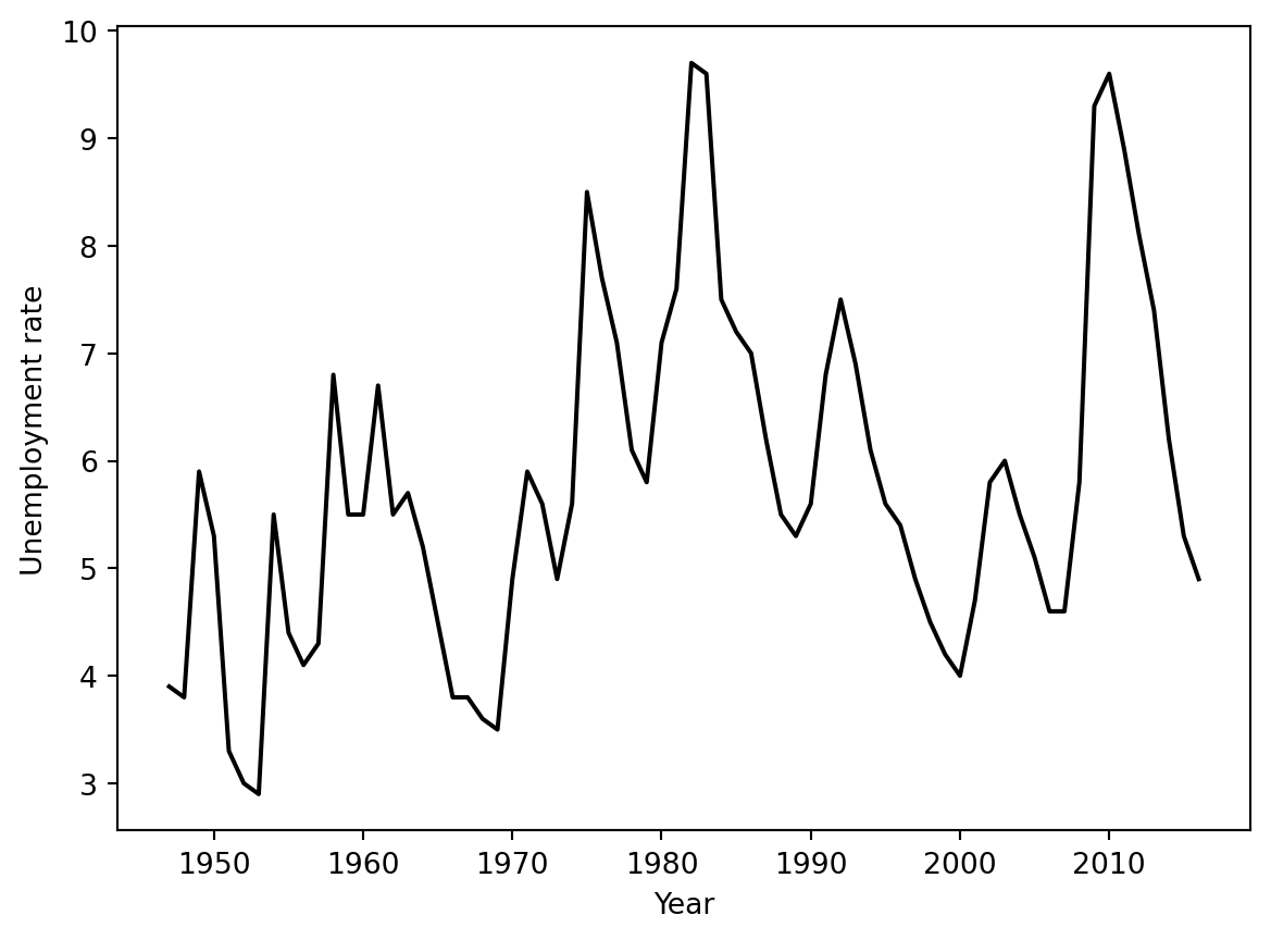
Plot the series

Code

fig, ax = plt.subplots()
ax.plot(unemp.year, unemp.y, color="black")
ax.set_xlabel("Year")
ax.set_ylabel("Unemployment rate")

Text(0, 0.5, 'Unemployment rate')

AR(1) fit

Code

unemp["y_lag"] = unemp.y.shift(1)
fit_lag = smf.ols("y ~ y_lag", data=unemp.dropna()).fit()
fit_lag.summary()

OLS Regression Results
Dep. Variable:	y	R-squared:	0.601
Model:	OLS	Adj. R-squared:	0.595
Method:	Least Squares	F-statistic:	100.7
Date:	Sun, 31 May 2026	Prob (F-statistic):	5.54e-15
Time:	23:05:54	Log-Likelihood:	-98.513
No. Observations:	69	AIC:	201.0
Df Residuals:	67	BIC:	205.5
Df Model:	1
Covariance Type:	nonrobust

	coef	std err	t	P>\|t\|	[0.025	0.975]
Intercept	1.3536	0.461	2.939	0.005	0.434	2.273
y_lag	0.7688	0.077	10.036	0.000	0.616	0.922

Omnibus:	20.288	Durbin-Watson:	1.582
Prob(Omnibus):	0.000	Jarque-Bera (JB):	26.717
Skew:	1.254	Prob(JB):	1.58e-06
Kurtosis:	4.733	Cond. No.	23.0

Notes:
[1] Standard Errors assume that the covariance matrix of the errors is correctly specified.

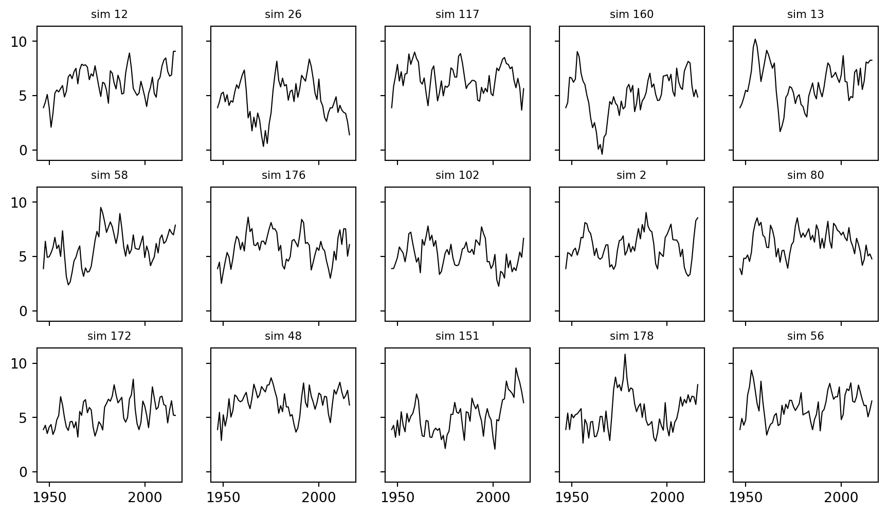
Simulate replicated series

Code

rng = np.random.default_rng(123)
n = len(unemp)
S = 200
sigma = np.sqrt(fit_lag.mse_resid)
a, b = fit_lag.params["Intercept"], fit_lag.params["y_lag"]
y_rep = np.empty((S, n))
y_rep[:, 0] = unemp.y.iloc[0]
for s in range(S):
    for t in range(1, n):
        y_rep[s, t] = a + b * y_rep[s, t-1] + rng.normal(0, sigma)

Code

fig, axs = plt.subplots(3, 5, figsize=(11, 6), sharex=True, sharey=True)
for ax, s in zip(axs.ravel(), rng.choice(S, 15, replace=False)):
    ax.plot(unemp.year, y_rep[s], color="black", linewidth=0.8)
    ax.set_title(f"sim {s}", fontsize=8)

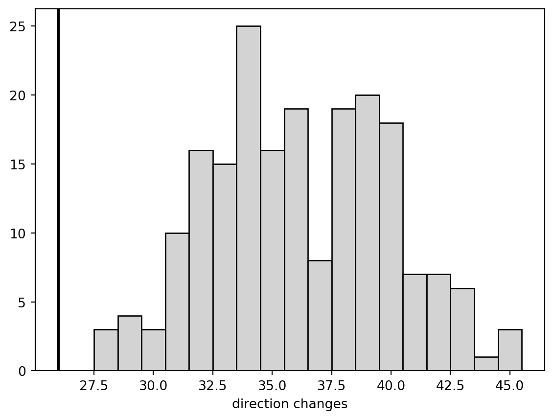
Test statistic: changes in direction

Code

def direction_changes(y):
    y = np.asarray(y)
    return np.sum(np.sign(y[2:] - y[1:-1]) != np.sign(y[1:-1] - y[:-2]))

test_y = direction_changes(unemp.y)
test_rep = np.apply_along_axis(direction_changes, 1, y_rep)
print(test_y, np.mean(test_rep > test_y), np.quantile(test_rep, [0.1, 0.5, 0.9]))

26 1.0 [31.9 36.  41. ]

Code

fig, ax = plt.subplots()
ax.hist(test_rep, bins=np.arange(test_rep.min(), test_rep.max()+2)-0.5, color="lightgray", edgecolor="black")
ax.axvline(test_y, color="black", linewidth=2)
ax.set_xlabel("direction changes")

Text(0.5, 0, 'direction changes')