# Robit and logit regression
Source: `Robit/robit.Rmd`
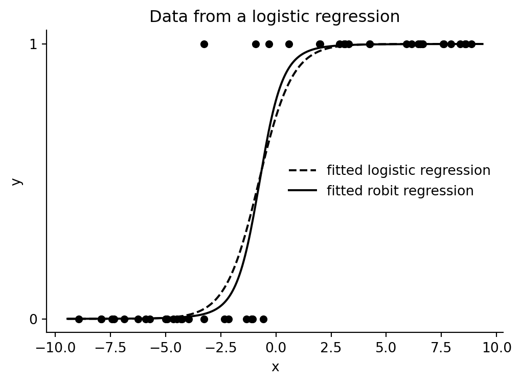
This example compares ordinary logistic regression with a robust binary-response model whose inverse link is a Student-t CDF. The heavier-tailed robit link is less distorted by a deliberately flipped low-`x` observation.
## Simulate data from a logit model
```{python}
from pathlib import Path
import numpy as np
import pandas as pd
import matplotlib.pyplot as plt
from scipy.special import expit
from scipy.stats import t
import statsmodels.api as sm

root = Path("../../ROS-Examples")
robit_dir = root / "Robit"

rng = np.random.default_rng(1234)
N = 50
x = rng.uniform(-9, 9, size=N)
a, b = 0.0, 0.8
p = expit(a + b * x)
y = rng.binomial(1, p)
df = 4.0
scale = np.sqrt((df - 2) / df)
data_1 = pd.DataFrame({"x": x, "y": y})
data_1.head()
```
## Frequentist logit baseline
```{python}
X = sm.add_constant(data_1["x"])
fit_logit_sm_1 = sm.Logit(data_1["y"], X).fit(disp=False)
fit_logit_sm_1.params
```
## Stan models via CmdStanPy
The two original Stan programs are:
```stan
// logit.stan
model {
  y ~ bernoulli_logit(a + b*x);
}
```
```stan
// robit.stan
model {
  vector[N] p;
  for (n in 1:N) p[n] = student_t_cdf(a + b*x[n], df, 0, sqrt((df - 2)/df));
  y ~ bernoulli(p);
}
```
```{python}
from cmdstanpy import CmdStanModel

stan_dir = Path("_generated_stan")
stan_dir.mkdir(exist_ok=True)
logit_stan = stan_dir / "robit_logit_modern.stan"
logit_stan.write_text(r'''
data {
  int<lower=1> N;
  vector[N] x;
  array[N] int<lower=0, upper=1> y;
}
parameters {
  real a;
  real b;
}
model {
  a ~ normal(0, 5);
  b ~ normal(0, 5);
  y ~ bernoulli_logit(a + b*x);
}
''')
robit_stan = stan_dir / "robit_modern.stan"
robit_stan.write_text(r'''
data {
  int<lower=1> N;
  vector[N] x;
  array[N] int<lower=0, upper=1> y;
  real<lower=2> df;
}
parameters {
  real a;
  real b;
}
model {
  vector[N] p;
  a ~ normal(0, 5);
  b ~ normal(0, 5);
  for (n in 1:N) p[n] = student_t_cdf(a + b*x[n] | df, 0, sqrt((df - 2)/df));
  y ~ bernoulli(p);
}
''')

logit_model = CmdStanModel(stan_file=str(logit_stan))
robit_model = CmdStanModel(stan_file=str(robit_stan))

def stan_data(frame):
    return {"N": len(frame), "x": frame.x.to_numpy(), "y": frame.y.astype(int).tolist(), "df": df}

fit_logit_1 = logit_model.sample(data={k: v for k, v in stan_data(data_1).items() if k != "df"}, seed=1507, chains=4, parallel_chains=4, show_progress=False)
fit_robit_1 = robit_model.sample(data=stan_data(data_1), seed=1507, chains=4, parallel_chains=4, show_progress=False)

med_logit_1 = fit_logit_1.draws_pd()[["a", "b"]].median()
med_robit_1 = fit_robit_1.draws_pd()[["a", "b"]].median()
med_logit_1, med_robit_1
```
## Plot the fitted links
```{python}
def robit_prob(x, a, b, df=df):
    return t.cdf(a + b * x, df=df, loc=0, scale=np.sqrt((df - 2) / df))

def plot_fits(frame, med_logit, med_robit, title):
    x_grid = np.linspace(frame.x.min() - 0.5, frame.x.max() + 0.5, 300)
    fig, ax = plt.subplots(figsize=(6, 4))
    ax.scatter(frame.x, frame.y, color="black", s=22)
    ax.plot(x_grid, expit(med_logit.a + med_logit.b * x_grid), color="black", ls="--", label="fitted logistic regression")
    ax.plot(x_grid, robit_prob(x_grid, med_robit.a, med_robit.b), color="black", label="fitted robit regression")
    ax.set(xlabel="x", ylabel="y", yticks=[0, 1], title=title)
    ax.legend(frameon=False, loc="center right")
    ax.spines[["top", "right"]].set_visible(False)

plot_fits(data_1, med_logit_1, med_robit_1, "Data from a logistic regression")
```
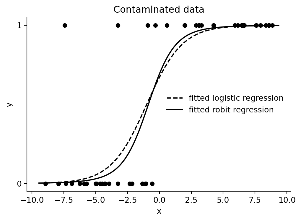
## Contaminate the data
The R code flips the fourth-smallest `x` value to `y = 1`, creating an outlying success far in the left tail.
```{python}
data_2 = data_1.copy()
low_idx = data_2["x"].sort_values().index[3]
data_2.loc[low_idx, "y"] = 1

fit_logit_2 = logit_model.sample(data={k: v for k, v in stan_data(data_2).items() if k != "df"}, seed=1508, chains=4, parallel_chains=4, show_progress=False)
fit_robit_2 = robit_model.sample(data=stan_data(data_2), seed=1508, chains=4, parallel_chains=4, show_progress=False)
med_logit_2 = fit_logit_2.draws_pd()[["a", "b"]].median()
med_robit_2 = fit_robit_2.draws_pd()[["a", "b"]].median()

plot_fits(data_2, med_logit_2, med_robit_2, "Contaminated data")
```
The logistic link tends to flatten to accommodate the flipped extreme case. The robit link can assign more tail probability to a single surprising point and preserve a steeper central transition.
## BlackJAX log-density sketch
The robit model is also a compact example of a custom Bernoulli likelihood. This function is the log density for parameters `(a, b)` with weak normal priors.
```{python}
from scipy.stats import norm as normal_dist, t as student_t

x_np = data_2.x.to_numpy()
y_np = data_2.y.to_numpy()

def robit_logdensity_ab(params):
    a, b = params["a"], params["b"]
    eta = (a + b * x_np) / scale
    p = np.clip(student_t.cdf(eta, df), 1e-9, 1 - 1e-9)
    ll = np.sum(y_np * np.log(p) + (1 - y_np) * np.log1p(-p))
    prior = normal_dist.logpdf(a, 0, 5) + normal_dist.logpdf(b, 0, 5)
    return ll + prior

robit_logdensity_ab({"a": med_robit_2["a"], "b": med_robit_2["b"]})
```