Code
import numpy as np
import pandas as pd
import matplotlib.pyplot as plt
from scipy.linalg import cho_factor, cho_solve
import statsmodels.api as sm

SEED = 1754
rng = np.random.default_rng(SEED)Source: FakeKCV/fake_kcv.Rmd
The original R example simulates 60 observations with 30 highly correlated predictors, then compares weak and shrinkage priors using PSIS-LOO and K-fold cross-validation. This Python port keeps the same data-generating setup and implements a conjugate Gaussian linear model so that posterior predictions can be evaluated directly. A strong but finite normal prior is used as a tractable analogue of the weakly informative prior; a tighter prior plays the role of global shrinkage.
import numpy as np
import pandas as pd
import matplotlib.pyplot as plt
from scipy.linalg import cho_factor, cho_solve
import statsmodels.api as sm
SEED = 1754
rng = np.random.default_rng(SEED)The predictors are correlated multivariate normal draws with pairwise correlation 0.8. Only the first three coefficients are nonzero.
n = 60
k = 30
rho = 0.8
sigma_y = 2.0
Sigma = rho * np.ones((k, k)) + (1 - rho) * np.eye(k)
X_raw = rng.multivariate_normal(np.zeros(k), Sigma, size=n)
beta_true = np.r_[-1, 1, 2, np.zeros(k - 3)]
y = X_raw @ beta_true + rng.normal(0, sigma_y, size=n)

columns = [f"x{j+1}" for j in range(k)]
fake = pd.DataFrame(X_raw, columns=columns)
fake["y"] = y
fake.head()| x1 | x2 | x3 | x4 | x5 | x6 | x7 | x8 | x9 | x10 | ... | x22 | x23 | x24 | x25 | x26 | x27 | x28 | x29 | x30 | y | |
|---|---|---|---|---|---|---|---|---|---|---|---|---|---|---|---|---|---|---|---|---|---|
| 0 | -0.408722 | -0.614240 | 0.503237 | 0.206527 | -0.024329 | -0.246085 | -0.510043 | -0.499994 | -0.601909 | -0.189147 | ... | -0.126521 | -0.032801 | -0.086618 | 0.309791 | -0.290005 | 0.219788 | -0.071657 | -0.439452 | -1.119990 | -0.084823 |
| 1 | 1.515684 | 0.641315 | 1.390885 | 1.797560 | 1.184903 | 1.358005 | 0.695008 | 1.063286 | 0.545237 | 1.051220 | ... | 1.033202 | 1.205759 | -0.053317 | 0.991851 | 0.980249 | 1.024671 | 0.884909 | 1.650005 | 1.028765 | 1.431682 |
| 2 | 1.515873 | 1.890154 | 1.169613 | 1.081623 | 1.202411 | 2.329621 | 1.510748 | 1.983054 | 2.596403 | 1.528695 | ... | 1.802543 | 0.595489 | 2.096685 | 1.419125 | 1.636324 | 2.020874 | 1.713995 | 1.073806 | 1.583208 | 5.133837 |
| 3 | 1.631458 | 0.507101 | 1.767810 | 1.826727 | 1.334866 | 1.854145 | 1.327120 | 1.746701 | 2.371878 | 1.467539 | ... | 1.663477 | 1.824545 | 2.024518 | 1.576733 | 2.042997 | 2.423548 | 1.687070 | 1.736297 | 1.372946 | 1.450625 |
| 4 | 0.881348 | 0.958295 | 1.192247 | 1.035403 | 0.337675 | -0.284381 | -0.071291 | 0.397053 | 0.801519 | 0.772577 | ... | 0.639218 | -0.255660 | 0.390349 | 0.953334 | 0.923226 | -0.408616 | -0.222284 | 0.372327 | 0.915308 | 0.057752 |
5 rows × 31 columns
ols = sm.OLS(fake["y"], sm.add_constant(fake[columns])).fit()
ols.params.head(), ols.rsquared
(const -0.020271
x1 -0.506902
x2 0.787774
x3 1.126856
x4 0.022589
dtype: float64,
np.float64(0.73019779043653))For a Gaussian likelihood with known residual scale, a normal prior on coefficients gives a normal posterior. The intercept is given a wide prior in both models; the slope prior scale controls shrinkage.
def add_intercept(X):
    return np.column_stack([np.ones(len(X)), np.asarray(X)])

X = add_intercept(fake[columns])


def posterior_normal(X_train, y_train, sigma=2.0, slope_prior_scale=10.0, intercept_prior_scale=100.0):
    p = X_train.shape[1]
    prior_var = np.r_[intercept_prior_scale**2, np.repeat(slope_prior_scale**2, p - 1)]
    prior_precision = np.diag(1 / prior_var)
    precision = prior_precision + X_train.T @ X_train / sigma**2
    rhs = X_train.T @ y_train / sigma**2
    cf = cho_factor(precision, lower=True, check_finite=False)
    cov = cho_solve(cf, np.eye(p), check_finite=False)
    mean = cov @ rhs
    return mean, cov


def predictive_logpdf(X_test, y_test, mean, cov, sigma=2.0):
    pred_mean = X_test @ mean
    pred_var = sigma**2 + np.sum((X_test @ cov) * X_test, axis=1)
    return -0.5 * (np.log(2 * np.pi * pred_var) + (y_test - pred_mean) ** 2 / pred_var)


def fit_and_score(slope_prior_scale):
    mean, cov = posterior_normal(X, y, sigma=sigma_y, slope_prior_scale=slope_prior_scale)
    elpd_in_sample = predictive_logpdf(X, y, mean, cov, sigma=sigma_y).sum()
    coef = pd.Series(mean[1:], index=columns, name="posterior_mean")
return mean, cov, elpd_in_sample, coefweak_mean, weak_cov, weak_lpd, weak_coef = fit_and_score(slope_prior_scale=10.0)
shrink_mean, shrink_cov, shrink_lpd, shrink_coef = fit_and_score(slope_prior_scale=0.5)
coef_compare = pd.DataFrame({
"true": beta_true,
"weak prior": weak_coef,
"shrinkage prior": shrink_coef,
})
coef_compare.head(10).round(2)| true | weak prior | shrinkage prior | |
|---|---|---|---|
| x1 | -1.0 | -0.50 | -0.05 |
| x2 | 1.0 | 0.79 | 0.46 |
| x3 | 2.0 | 1.13 | 0.79 |
| x4 | 0.0 | 0.02 | 0.05 |
| x5 | 0.0 | -0.72 | -0.49 |
| x6 | 0.0 | -0.82 | -0.10 |
| x7 | 0.0 | -0.24 | 0.06 |
| x8 | 0.0 | 1.96 | 0.40 |
| x9 | 0.0 | -0.64 | 0.03 |
| x10 | 0.0 | 1.17 | 0.25 |
fig, ax = plt.subplots(figsize=(7, 3.5))
ax.axhline(0, color="0.8", linewidth=1)
ax.plot(np.arange(1, k + 1), beta_true, "o", label="true")
ax.plot(np.arange(1, k + 1), weak_coef, "o", label="weak prior", alpha=0.75)
ax.plot(np.arange(1, k + 1), shrink_coef, "o", label="shrinkage prior", alpha=0.75)
ax.set_xlabel("coefficient index")
ax.set_ylabel("coefficient")
ax.legend(frameon=False)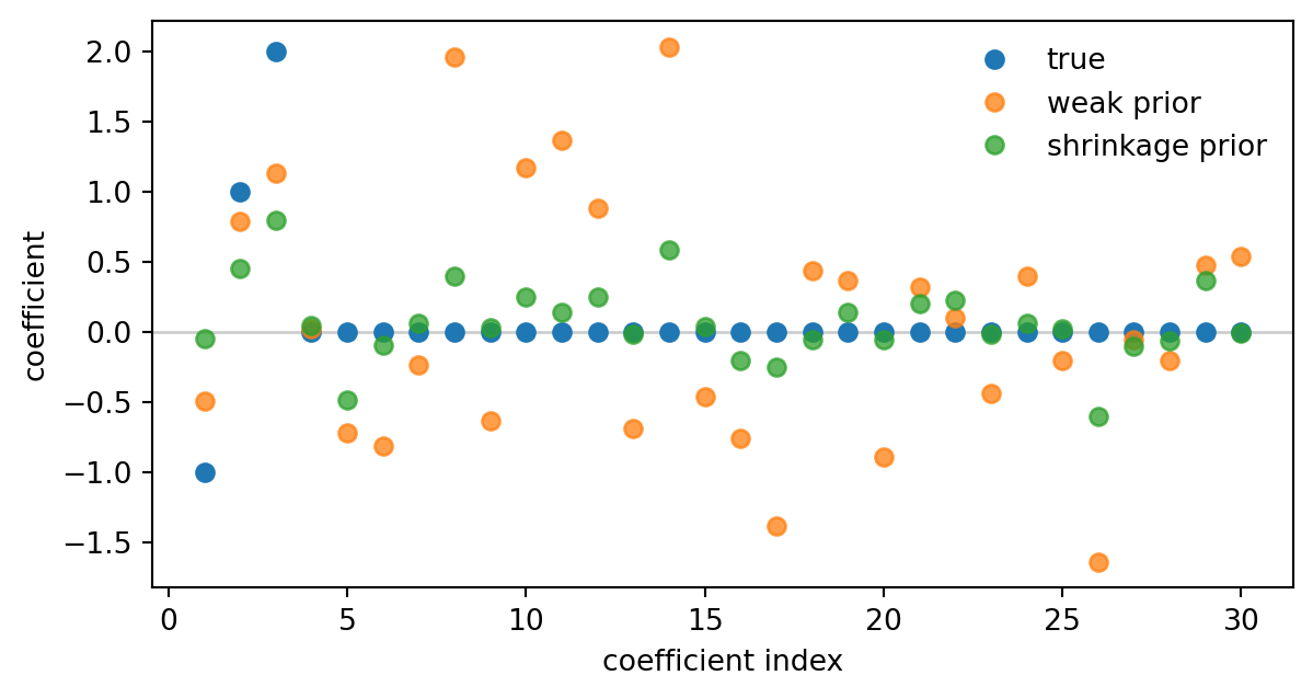
With many correlated predictors and only 60 observations, the weak-prior fit spreads signal across noise variables. The shrinkage prior pulls most coefficients closer to zero while preserving the largest signals.
The R example emphasizes that PSIS-LOO can be fragile here. Instead of implementing Pareto smoothing, this port computes exact refits for LOO and for 10-fold CV using the closed-form posterior. The K-fold estimate is noisier than exact LOO but follows the same predictive target.
def exact_loo_elpd(slope_prior_scale):
    parts = []
    for i in range(n):
        train = np.arange(n) != i
        mean, cov = posterior_normal(X[train], y[train], sigma=sigma_y, slope_prior_scale=slope_prior_scale)
        parts.append(predictive_logpdf(X[~train], y[~train], mean, cov, sigma=sigma_y)[0])
    return np.array(parts)


def kfold_elpd(slope_prior_scale, folds=10, rng=None):
    rng = np.random.default_rng(SEED) if rng is None else rng
    fold_id = np.tile(np.arange(folds), int(np.ceil(n / folds)))[:n]
    rng.shuffle(fold_id)
    parts = np.empty(n)
    for fold in range(folds):
        test = fold_id == fold
        mean, cov = posterior_normal(X[~test], y[~test], sigma=sigma_y, slope_prior_scale=slope_prior_scale)
        parts[test] = predictive_logpdf(X[test], y[test], mean, cov, sigma=sigma_y)
    return parts, fold_id

loo_weak = exact_loo_elpd(10.0)
loo_shrink = exact_loo_elpd(0.5)
kfold_weak, fold_id = kfold_elpd(10.0, folds=10, rng=np.random.default_rng(SEED))
kfold_shrink, _ = kfold_elpd(0.5, folds=10, rng=np.random.default_rng(SEED))cv_summary = pd.DataFrame({
"model": ["weak prior", "shrinkage prior"],
"in_sample_lpd": [weak_lpd, shrink_lpd],
"exact_loo_elpd": [loo_weak.sum(), loo_shrink.sum()],
"kfold_elpd": [kfold_weak.sum(), kfold_shrink.sum()],
})
cv_summary.assign(
loo_difference=lambda d: d["exact_loo_elpd"] - d.loc[d.model == "weak prior", "exact_loo_elpd"].iloc[0],
kfold_difference=lambda d: d["kfold_elpd"] - d.loc[d.model == "weak prior", "kfold_elpd"].iloc[0],
).round(1)| model | in_sample_lpd | exact_loo_elpd | kfold_elpd | loo_difference | kfold_difference | |
|---|---|---|---|---|---|---|
| 0 | weak prior | -119.4 | -150.1 | -150.3 | 0.0 | 0.0 |
| 1 | shrinkage prior | -121.4 | -133.0 | -134.9 | 17.1 | 15.4 |
pointwise = pd.DataFrame({
    "weak prior": loo_weak,
    "shrinkage prior": loo_shrink,
    "fold": fold_id,
})
pointwise["difference"] = pointwise["shrinkage prior"] - pointwise["weak prior"]
pointwise["difference"].describe(percentiles=[0.1, 0.5, 0.9]).round(2)
count 60.00
mean 0.28
std 0.51
min -1.04
10% -0.18
50% 0.23
90% 0.90
max 1.68
Name: difference, dtype: float64fig, ax = plt.subplots(figsize=(6, 3.5))
ax.scatter(pointwise["weak prior"], pointwise["shrinkage prior"], c=pointwise["fold"], cmap="tab10", s=35)
lo = min(pointwise["weak prior"].min(), pointwise["shrinkage prior"].min())
hi = max(pointwise["weak prior"].max(), pointwise["shrinkage prior"].max())
ax.plot([lo, hi], [lo, hi], color="black", linestyle="--", linewidth=1)
ax.set_xlabel("LOO log predictive density: weak prior")
ax.set_ylabel("LOO log predictive density: shrinkage prior")
ax.set_title("Pointwise exact LOO comparison")Text(0.5, 1.0, 'Pointwise exact LOO comparison')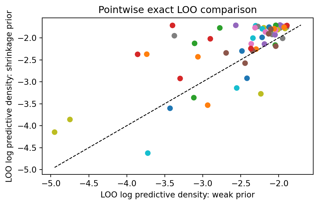
The predictive comparison favors shrinkage because the data-generating process is sparse. That is the same substantive lesson as the R version: with many correlated predictors and weak information in the likelihood, predictive validation can reveal overfitting, and a better regularizing prior can improve out-of-sample predictions.