# National Election Study: repeated linear regressions
Source: `NES/nes_linear.Rmd`
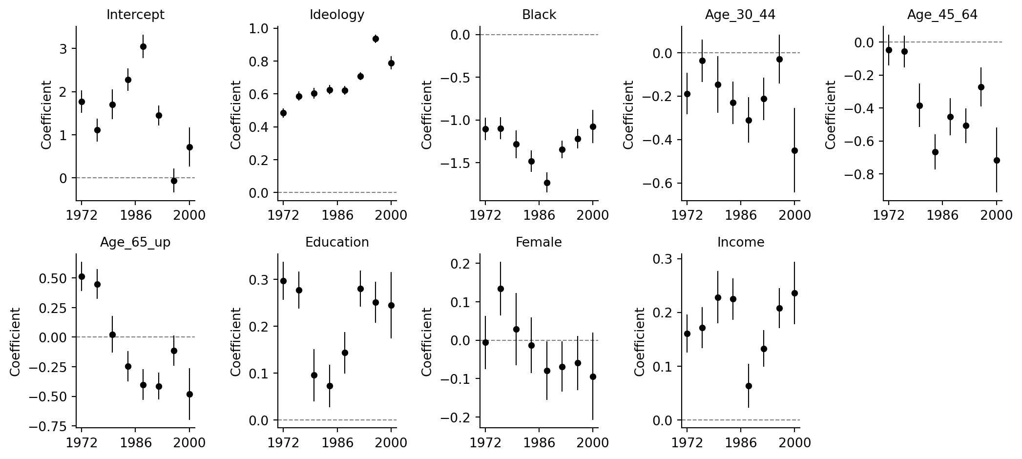
The ROS example fits the same party-identification regression separately in each presidential election year from 1972 through 2000. The coefficients are then plotted as a small multiple to show how a "secret weapon" workflow can summarize many related regressions.
## Setup and data
```{python}
from pathlib import Path
import numpy as np
import pandas as pd
import matplotlib.pyplot as plt
import statsmodels.formula.api as smf

root = Path("../../ROS-Examples")
nes_dir = root / "NES"
nes = pd.read_csv(nes_dir / "data/nes.txt", sep=r"\s+", index_col=0, na_values=["NA"])
nes.head()
```
## Fit the same model year by year
The R formula is
```text
partyid7 ~ real_ideo + race_adj + factor(age_discrete) + educ1 + female + income
```
In Python, `C(age_discrete)` gives the same treatment of the age group as a categorical predictor. We use ordinary least squares as the close frequentist analogue to the default Gaussian `stan_glm` fit in the source example.
```{python}
formula = "partyid7 ~ real_ideo + race_adj + C(age_discrete) + educ1 + female + income"
years = list(range(1972, 2001, 4))

rows = []
for year in years:
    this_year = nes.loc[nes["year"] == year].copy()
    fit = smf.ols(formula, data=this_year).fit()
    for name, coef in fit.params.items():
        rows.append({"year": year, "term": name, "coef": coef, "se": fit.bse[name], "nobs": fit.nobs})

coef_by_year = pd.DataFrame(rows)
coef_by_year.head()
```
The original figure uses readable labels for the nine displayed coefficients. Patsy names the categorical age terms according to the observed coding in `age_discrete`; the mapping below mirrors the book labels.
```{python}
term_labels = {
    "Intercept": "Intercept",
    "real_ideo": "Ideology",
    "race_adj": "Black",
    "C(age_discrete)[T.2]": "Age_30_44",
    "C(age_discrete)[T.3]": "Age_45_64",
    "C(age_discrete)[T.4]": "Age_65_up",
    "educ1": "Education",
    "female": "Female",
    "income": "Income",
}
plot_df = coef_by_year.loc[coef_by_year["term"].isin(term_labels)].copy()
plot_df["label"] = plot_df["term"].map(term_labels)
plot_df["lo"] = plot_df["coef"] - 0.67 * plot_df["se"]
plot_df["hi"] = plot_df["coef"] + 0.67 * plot_df["se"]
plot_df.sort_values(["label", "year"]).head()
```
## Coefficient plot
The bars are plus/minus `0.67` standard errors, matching the R page. This interval corresponds roughly to a 50% uncertainty interval under a normal approximation, which makes it visually less cluttered than 95% intervals in a small multiple plot.
```{python}
labels = list(term_labels.values())
fig, axes = plt.subplots(2, 5, figsize=(11, 5), sharex=False)
axes = axes.ravel()

for ax, label in zip(axes, labels):
    d = plot_df.loc[plot_df["label"] == label].sort_values("year")
    ax.axhline(0, color="0.5", ls="--", lw=0.8)
    ax.errorbar(d["year"], d["coef"], yerr=0.67 * d["se"], fmt="o", color="black", ms=4, lw=0.8)
    ax.set_title(label, fontsize=10)
    ax.set_xticks([1972, 1986, 2000])
    ax.set_ylabel("Coefficient")
    ax.spines[["top", "right"]].set_visible(False)

axes[-1].axis("off")
fig.tight_layout()
```
## Bayesian version with CmdStanPy
A direct CmdStanPy port is useful if exact posterior uncertainty is desired. The model is just Gaussian regression with a design matrix assembled by Patsy. Run it inside the loop above to replace `fit.params` and `fit.bse` with posterior medians and posterior standard deviations.
```{python}
import patsy
from cmdstanpy import CmdStanModel

stan_code = """
data {
  int<lower=1> N;
  int<lower=1> K;
  matrix[N, K] X;
  vector[N] y;
}
parameters {
  vector[K] beta;
  real<lower=0> sigma;
}
model {
  beta ~ normal(0, 10);
  sigma ~ exponential(1);
  y ~ normal(X * beta, sigma);
}
"""
stan_file = Path("_generated/nes_linear_regression.stan")
stan_file.parent.mkdir(exist_ok=True)
stan_file.write_text(stan_code)

sample_year = nes.loc[nes["year"] == 1972].copy()
y_mat, x_mat = patsy.dmatrices(formula, sample_year, return_type="dataframe")
model = CmdStanModel(stan_file=str(stan_file))
fit = model.sample(
    data={"N": x_mat.shape[0], "K": x_mat.shape[1], "X": x_mat.to_numpy(), "y": y_mat.iloc[:, 0].to_numpy()},
    seed=1972,
    chains=4,
    parallel_chains=4,
    show_progress=False,
)
posterior = fit.draws_pd()
posterior.filter(regex=r"^beta\[").describe(percentiles=[0.05, 0.5, 0.95])
```