Metabolic rate and body mass

Source: Metabolic/metabolic.Rmd

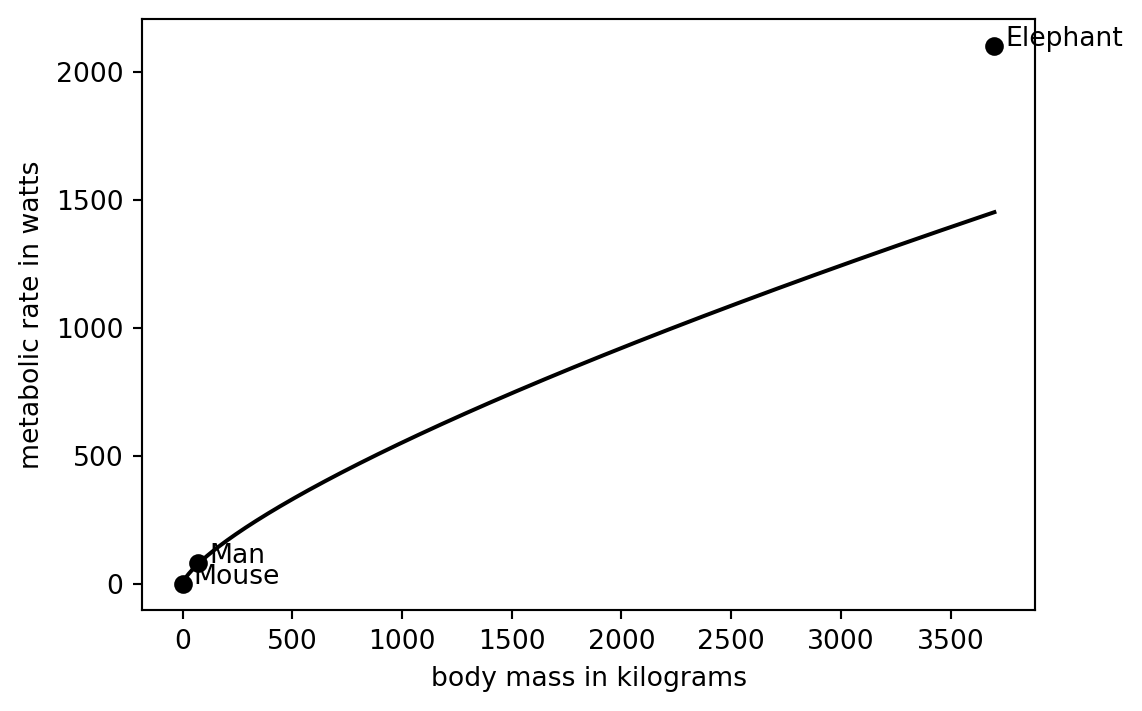
This example illustrates how to interpret a power-law regression. A linear relation on the log scale, \(\log y = 1.2 + 0.74\log x\), corresponds to the nonlinear curve \(y = \exp(1.2)x^{0.74}\) on the original scale.

Code

import numpy as np
import matplotlib.pyplot as plt

animals = {
    "Mouse": (0.02, 0.17),
    "Man": (70, 80),
    "Elephant": (3700, 2100),
}

Log-log view

Code

xs = np.linspace(np.log(.01), np.log(3000), 200)
fig, ax = plt.subplots(figsize=(6, 4))
ax.plot(xs, 1.2 + 0.74*xs, color="black")
for label, (mass, rate) in animals.items():
    ax.scatter(np.log(mass), np.log(rate), color="black")
    ax.text(np.log(mass)+0.15, np.log(rate), label)
ax.set_xlabel("log body mass in kilograms")
ax.set_ylabel("log metabolic rate in watts")
ax.grid(color="lightgray")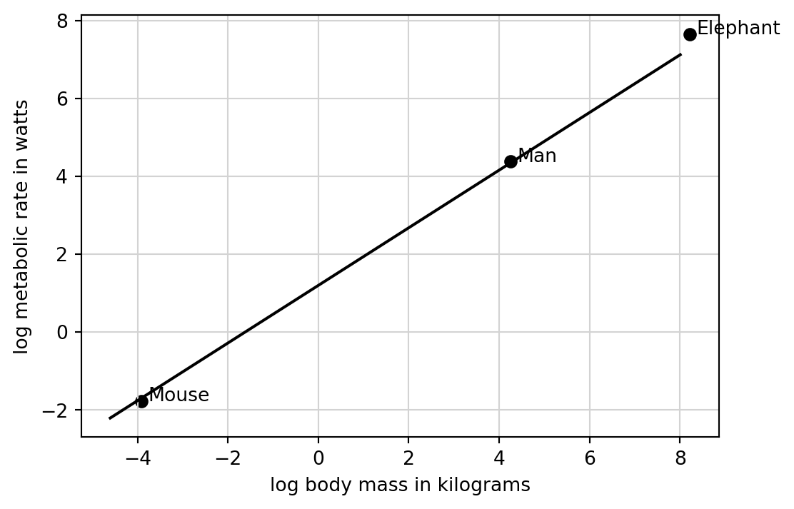

Original-scale view

Code

x = np.linspace(0.01, 3700, 400)
y = np.exp(1.2 + 0.74*np.log(x))
fig, ax = plt.subplots(figsize=(6, 4))
ax.plot(x, y, color="black")
for label, (mass, rate) in animals.items():
    ax.scatter(mass, rate, color="black")
    ax.text(mass + 50, rate, label)
ax.set_xlabel("body mass in kilograms")
ax.set_ylabel("metabolic rate in watts")

Text(0, 0.5, 'metabolic rate in watts')