Baby names: popularity, timing, and volatility

Source: Names/names.Rmd

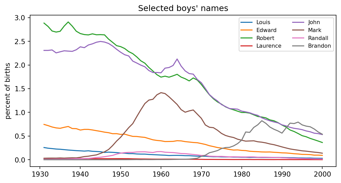
This page ports the core name-statistics workflow: normalize name counts by year, compute timing/popularity/volatility summaries, and display selected names ordered by peak year.

Code

from pathlib import Path
import numpy as np
import pandas as pd
import matplotlib.pyplot as plt
import statsmodels.api as sm

root = Path("../../ROS-Examples")
allnames = pd.read_csv(root / "Names/data/allnames_clean.csv")
allnames.head()

	X	name	sex	X1880	X1881	X1882	X1883	X1884	X1885	X1886	...	X2001	X2002	X2003	X2004	X2005	X2006	X2007	X2008	X2009	X2010
0	1	Mary	F	7065	6919	8149	8012	9217	9128	9891	...	5715	5439	4996	4792	4439	4073	3665	3478	3132	2826
1	2	Anna	F	2604	2698	3143	3306	3860	3994	4283	...	10564	10372	9429	9510	9085	8590	7866	7236	6755	6242
2	3	Emma	F	2003	2034	2303	2367	2587	2728	2764	...	13299	16520	22690	21591	20318	19092	18338	18765	17830	17179
3	4	Elizabeth	F	1939	1852	2187	2255	2549	2582	2680	...	14767	14581	14083	13536	12705	12397	13013	11956	10969	10135
4	5	Minnie	F	1746	1653	2004	2035	2243	2178	2372	...	25	33	25	26	31	37	17	43	28	37

5 rows × 134 columns

Normalize counts by year

Code

years = np.arange(1931, 2001)
year_cols = [f"X{y}" for y in years]
counts = allnames[year_cols].to_numpy(dtype=float)
counts_norm = counts / counts.sum(axis=0, keepdims=True)
counts_adj = np.where(counts == 0, 2, counts)
counts_adj_norm = counts_adj / counts_adj.sum(axis=0, keepdims=True)

Compute per-name statistics

Code

def slope_for(logcounts, mask):
    X = sm.add_constant(years[mask] / 10)
    return sm.OLS(logcounts[mask], X).fit().params[1]

stats = []
for i, row in allnames.iterrows():
    cn = counts_norm[i]
    ca = counts_adj_norm[i]
    if cn.sum() == 0:
        continue
    logc = np.log(ca)
    stats.append({
        "name": row["name"],
        "sex": row["sex"],
        "avg_year": np.sum(years * counts[i]) / max(counts[i].sum(), 1),
        "avg_pop": cn.mean(),
        "max_pop": cn.max(),
        "ratio": ca.max() / ca.min(),
        "year_of_max_pop": years[np.argmax(cn)],
        "volatility": logc.std(ddof=1),
        "slope_1931_2000": slope_for(logc, np.ones_like(years, dtype=bool)),
        "slope_1981_2000": slope_for(logc, years >= 1981),
        "pop_2000": cn[-1],
    })
stats = pd.DataFrame(stats)
stats.head()

	name	sex	avg_year	avg_pop	max_pop	ratio	year_of_max_pop	volatility	slope_1931_2000	slope_1981_2000	pop_2000
0	Mary	F	1952.637594	0.011486	0.028763	16.789334	1931	0.985304	-0.475937	-0.305791	0.001637
1	Anna	F	1968.114234	0.001645	0.004020	3.955242	1931	0.367183	-0.004815	0.304544	0.002802
2	Emma	F	1971.736808	0.000708	0.003322	24.532850	2000	0.942119	-0.066410	1.728734	0.003322
3	Elizabeth	F	1968.830722	0.004552	0.005867	1.609374	1982	0.122865	0.030649	-0.212757	0.003997
4	Minnie	F	1945.203178	0.000192	0.000858	128.831756	1932	1.564222	-0.761433	-0.360689	0.000008

Sample names and display summary columns

Code

rng = np.random.default_rng(123)
def sample_names(sex, n=30):
    sub = stats[stats.sex == sex]
    p = sub.avg_pop.to_numpy()
    p = p / p.sum()
    take = rng.choice(sub.index, size=n, replace=False, p=p)
    out = sub.loc[take].sort_values("year_of_max_pop")
    return out[["name", "year_of_max_pop", "avg_year", "max_pop", "ratio", "slope_1931_2000", "slope_1981_2000", "pop_2000"]]

sample_names("F", 20)

	name	year_of_max_pop	avg_year	max_pop	ratio	slope_1931_2000	slope_1981_2000	pop_2000
132	Evelyn	1931	1953.352123	0.004050	15.583576	-0.359272	0.289174	0.000589
135	Betty	1931	1944.082911	0.017210	358.513630	-0.912142	-0.754725	0.000046
1095	Joyce	1941	1948.510926	0.006449	68.995351	-0.745439	-0.432684	0.000096
162	Carolyn	1942	1953.057370	0.007335	29.138282	-0.469936	-0.441137	0.000272
2991	Sharon	1943	1955.282121	0.008775	48.249333	-0.437494	-0.642967	0.000178
1076	Rosemary	1946	1952.775878	0.001407	14.880561	-0.443086	-0.231504	0.000104
2380	Janice	1946	1952.264707	0.004402	53.551224	-0.618689	-0.651632	0.000082
111	Theresa	1961	1960.588685	0.002896	16.007323	-0.260992	-0.807580	0.000180
217	Teresa	1962	1963.657168	0.004596	19.188583	-0.041046	-0.684874	0.000238
6761	Jody	1970	1967.063844	0.000612	83.131031	0.168681	-1.315361	0.000018
9744	Tara	1972	1979.555568	0.002306	2611.329327	1.099735	-0.958911	0.000354
6316	Jolene	1974	1968.394721	0.000347	13.877198	0.039346	-1.004571	0.000039
5805	Jennifer	1974	1977.791538	0.020812	1802.153938	0.913834	-1.081952	0.002488
7175	Robyn	1974	1972.497209	0.000526	227.159053	0.534176	-0.727523	0.000093
107	Amy	1975	1975.389977	0.010711	72.810635	0.509125	-1.105964	0.000840
4364	Shannon	1976	1978.897541	0.004417	416.006553	0.803232	-0.660408	0.000577
9	Sarah	1981	1979.619570	0.008169	8.721920	0.304763	-0.261031	0.004686
147	Victoria	1993	1977.659394	0.003435	14.650281	0.307785	0.622317	0.002895
12107	Alyssa	1999	1992.619375	0.003806	7664.080337	1.536104	1.392605	0.003592
11909	Giselle	2000	1989.653013	0.000394	716.459120	0.896072	1.105862	0.000394

Popularity trajectories for selected names

Code

selected = sample_names("M", 12)["name"].tolist()[:8]
fig, ax = plt.subplots(figsize=(8, 4))
for name in selected:
    idx = allnames.index[(allnames.name == name) & (allnames.sex == "M")][0]
    ax.plot(years, 100*counts_norm[idx], label=name)
ax.set_ylabel("percent of births")
ax.set_title("Selected boys' names")
ax.legend(ncol=2, fontsize=8)

# Baby names: popularity, timing, and volatility Source: `Names/names.Rmd` This page ports the core name-statistics workflow: normalize name counts by year, compute timing/popularity/volatility summaries, and display selected names ordered by peak year. ```{python} from pathlib import Path import numpy as np import pandas as pd import matplotlib.pyplot as plt import statsmodels.api as sm root = Path("../../ROS-Examples") allnames = pd.read_csv(root / "Names/data/allnames_clean.csv") allnames.head() ``` ## Normalize counts by year ```{python} years = np.arange(1931, 2001) year_cols = [f"X{y}" for y in years] counts = allnames[year_cols].to_numpy(dtype=float) counts_norm = counts / counts.sum(axis=0, keepdims=True) counts_adj = np.where(counts == 0, 2, counts) counts_adj_norm = counts_adj / counts_adj.sum(axis=0, keepdims=True) ``` ## Compute per-name statistics ```{python} def slope_for(logcounts, mask): X = sm.add_constant(years[mask] / 10) return sm.OLS(logcounts[mask], X).fit().params[1] stats = [] for i, row in allnames.iterrows(): cn = counts_norm[i] ca = counts_adj_norm[i] if cn.sum() == 0: continue logc = np.log(ca) stats.append({ "name": row["name"], "sex": row["sex"], "avg_year": np.sum(years * counts[i]) / max(counts[i].sum(), 1), "avg_pop": cn.mean(), "max_pop": cn.max(), "ratio": ca.max() / ca.min(), "year_of_max_pop": years[np.argmax(cn)], "volatility": logc.std(ddof=1), "slope_1931_2000": slope_for(logc, np.ones_like(years, dtype=bool)), "slope_1981_2000": slope_for(logc, years >= 1981), "pop_2000": cn[-1], }) stats = pd.DataFrame(stats) stats.head() ``` ## Sample names and display summary columns ```{python} rng = np.random.default_rng(123) def sample_names(sex, n=30): sub = stats[stats.sex == sex] p = sub.avg_pop.to_numpy() p = p / p.sum() take = rng.choice(sub.index, size=n, replace=False, p=p) out = sub.loc[take].sort_values("year_of_max_pop") return out[["name", "year_of_max_pop", "avg_year", "max_pop", "ratio", "slope_1931_2000", "slope_1981_2000", "pop_2000"]] sample_names("F", 20) ``` ## Popularity trajectories for selected names ```{python} selected = sample_names("M", 12)["name"].tolist()[:8] fig, ax = plt.subplots(figsize=(8, 4)) for name in selected: idx = allnames.index[(allnames.name == name) & (allnames.sex == "M")][0] ax.plot(years, 100*counts_norm[idx], label=name) ax.set_ylabel("percent of births") ax.set_title("Selected boys' names") ax.legend(ncol=2, fontsize=8) ```