# Congress / predictive uncertainty
Source: `Congress/congress.Rmd`
This page ports the congressional-election example from **Regression and Other Stories**. The original uses `rstanarm::stan_glm` to fit a Gaussian regression for Democratic two-party vote share in 1988, then propagates posterior predictive uncertainty to the 1990 House elections. The Python version keeps `statsmodels` for least-squares summaries and uses the lightweight Bayesian linear-regression helper for posterior predictive simulation.
## Setup and data
```{python}
from pathlib import Path
import numpy as np
import pandas as pd
import matplotlib.pyplot as plt
import statsmodels.formula.api as smf
from python.bayes_glm import bayes_lm


def ros_root():
    candidates = [
        Path("../../ROS-Examples"),
        Path("../ROS-Examples"),
        Path("/Users/alal/tmp/ros-python-book/ROS-Examples"),
    ]
    for candidate in candidates:
        if candidate.exists():
            return candidate
    return candidates[0]

root = ros_root()
congress = pd.read_csv(root / "Congress/data/congress.csv")
congress.head()
```
```{python}
congress[["v86", "v88", "v90", "v86_adj", "v88_adj", "v90_adj", "inc88", "inc90"]].describe()
```
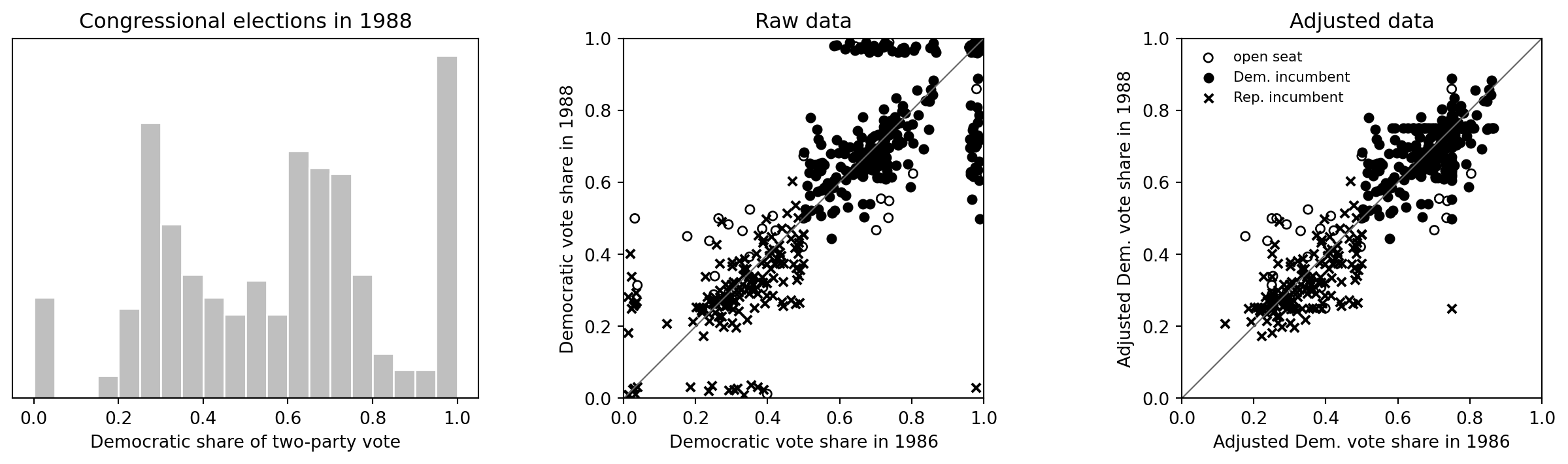
The raw vote shares contain uncontested races coded near 0 or 1. The adjusted variables keep the same substantive scale but are better suited for the linear regression used in the book.
## Predict 1988 vote from 1986 vote and incumbency
```{python}
data88 = congress.rename(columns={"v88_adj": "vote", "v86_adj": "past_vote", "inc88": "inc"})
fit88 = smf.ols("vote ~ past_vote + inc", data=data88).fit()
fit88_bayes = bayes_lm("vote ~ past_vote + inc", data=data88, draws=4000, prior_scale=10.0, seed=84735)
fit88.summary()
```
```{python}
coef_table = pd.DataFrame({
    "estimate": fit88.params,
    "std_error": fit88.bse,
    "t": fit88.tvalues,
})
coef_table
```
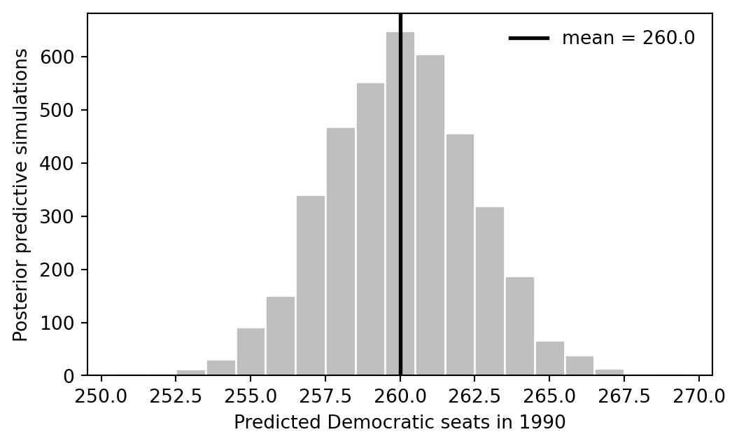
## Predict the 1990 election district by district
The R code calls `posterior_predict(fit88, newdata=data90)`. For this Gaussian linear model the helper draws coefficients and residual scale from the conjugate posterior and then generates replicated 1990 vote shares.
```{python}
rng = np.random.default_rng(84735)
data90 = pd.DataFrame({
    "past_vote": congress["v88_adj"],
    "inc": congress["inc90"],
})
pred90 = fit88_bayes.predict(data90, seed=84736)
dems_pred = (pred90 > 0.5).sum(axis=1)

pd.Series(dems_pred).describe()[["mean", "std", "min", "25%", "50%", "75%", "max"]]
```
```{python}
fig, ax = plt.subplots(figsize=(6, 3.5))
ax.hist(dems_pred, bins=np.arange(dems_pred.min() - 0.5, dems_pred.max() + 1.5), color="0.75", edgecolor="white")
ax.axvline(dems_pred.mean(), color="black", linewidth=2, label=f"mean = {dems_pred.mean():.1f}")
ax.set_xlabel("Predicted Democratic seats in 1990")
ax.set_ylabel("Posterior predictive simulations")
ax.legend(frameon=False)
```
## Vote-share graphics
```{python}
def jitter_extremes(vote, rng, low=0.1, high=0.9):
    vote = np.asarray(vote)
    out = vote.astype(float).copy()
    out[vote < low] = rng.uniform(0.01, 0.04, size=(vote < low).sum())
    out[vote > high] = rng.uniform(0.96, 0.99, size=(vote > high).sum())
    return out

fig, axes = plt.subplots(1, 3, figsize=(13, 3.8))

v88_hist = congress["v88"].clip(0.0001, 0.9999)
axes[0].hist(v88_hist, bins=np.arange(0, 1.05, 0.05), color="0.75", edgecolor="white")
axes[0].set_xlabel("Democratic share of two-party vote")
axes[0].set_yticks([])
axes[0].set_title("Congressional elections in 1988")

j_v86 = jitter_extremes(congress["v86"], rng)
j_v88 = jitter_extremes(congress["v88"], rng)
for inc, marker, label in [(0, "o", "open seat"), (1, "o", "Dem. incumbent"), (-1, "x", "Rep. incumbent")]:
    ok = congress["inc88"] == inc
    kwargs = {"s": 25, "label": label}
    if inc == 0:
        axes[1].scatter(j_v86[ok], j_v88[ok], facecolors="none", edgecolors="black", **kwargs)
    elif inc == 1:
        axes[1].scatter(j_v86[ok], j_v88[ok], color="black", marker=marker, **kwargs)
    else:
        axes[1].scatter(j_v86[ok], j_v88[ok], color="black", marker=marker, **kwargs)
axes[1].plot([0, 1], [0, 1], color="0.4", linewidth=0.8)
axes[1].set_xlabel("Democratic vote share in 1986")
axes[1].set_ylabel("Democratic vote share in 1988")
axes[1].set_title("Raw data")

for inc, marker, label in [(0, "o", "open seat"), (1, "o", "Dem. incumbent"), (-1, "x", "Rep. incumbent")]:
    ok = congress["inc88"] == inc
    if inc == 0:
        axes[2].scatter(congress.loc[ok, "v86_adj"], congress.loc[ok, "v88_adj"], facecolors="none", edgecolors="black", s=25, label=label)
    elif inc == 1:
        axes[2].scatter(congress.loc[ok, "v86_adj"], congress.loc[ok, "v88_adj"], color="black", s=25, label=label)
    else:
        axes[2].scatter(congress.loc[ok, "v86_adj"], congress.loc[ok, "v88_adj"], color="black", marker=marker, s=25, label=label)
axes[2].plot([0, 1], [0, 1], color="0.4", linewidth=0.8)
axes[2].set_xlabel("Adjusted Dem. vote share in 1986")
axes[2].set_ylabel("Adjusted Dem. vote share in 1988")
axes[2].set_title("Adjusted data")
axes[2].legend(frameon=False, fontsize=8)

for ax in axes[1:]:
    ax.set_xlim(0, 1)
    ax.set_ylim(0, 1)
    ax.set_aspect("equal", adjustable="box")
fig.tight_layout()
```
## CmdStanPy analogue
`rstanarm::stan_glm` supplies weakly informative priors automatically. A direct CmdStanPy version is useful if the prior needs to be explicit; for the book's predictive calculation, the helper fit above reproduces the core posterior-predictive workflow without requiring Stan at render time.
```{python}
#| eval: false
from cmdstanpy import CmdStanModel

# A minimal Stan model would put normal priors on alpha/beta and a half-normal
# prior on sigma, then generate y_rep for the 1990 design matrix in
# generated quantities.  Compile and sample it only when exact prior matching is
# important for the exercise.
```