# Congress / historical vote-swing plots
Source: `Congress/congress_plots.Rmd`
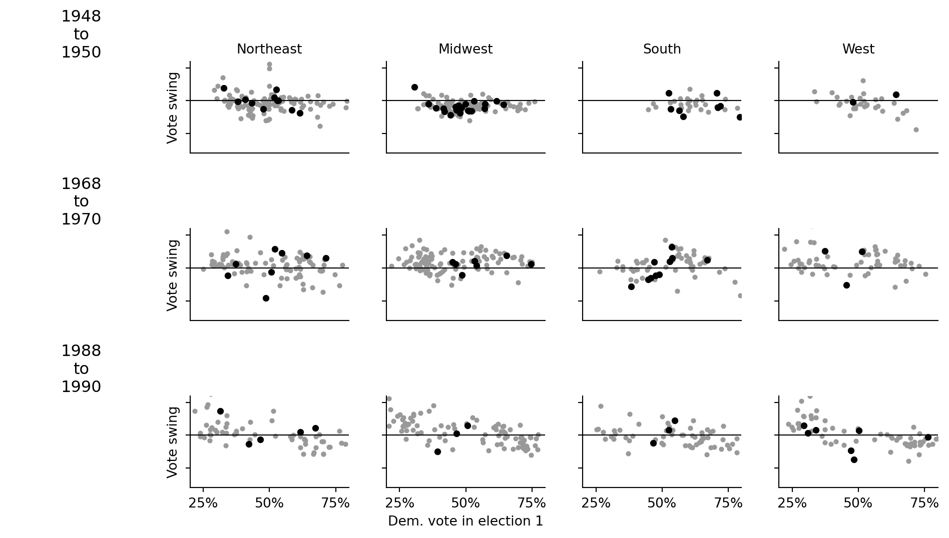
This example builds the Chapter 2 congressional vote-swing grid: for selected elections, compare Democratic vote in election 1 to the swing in election 2, faceted by region. The original data files are fixed-width-ish numeric `.asc` files; each row contains district identifiers, incumbency, and the two-party vote counts.
## Load and stack the biennial files
```{python}
from pathlib import Path
import numpy as np
import pandas as pd
import matplotlib.pyplot as plt


def ros_root():
    candidates = [
        Path("../../ROS-Examples"),
        Path("../ROS-Examples"),
        Path("/Users/alal/tmp/ros-python-book/ROS-Examples"),
    ]
    for candidate in candidates:
        if candidate.exists():
            return candidate
    return candidates[0]

root = ros_root()
congress_dir = root / "Congress/data"
region_name = ["Northeast", "Midwest", "South", "West"]

def read_congress_year(year):
    arr = np.loadtxt(congress_dir / f"{year}.asc")
    df = pd.DataFrame(arr, columns=["state_code", "district", "inc", "dem_votes", "rep_votes"])
    df.insert(0, "year", year)
    return df

congress_by_year = {year: read_congress_year(year) for year in range(1896, 1993, 2)}
congress_by_year[1988].head()
```
## Build pairwise vote-swing data
```{python}
def election_pair(first_year):
    first = congress_by_year[first_year].copy().reset_index(drop=True)
    second = congress_by_year[first_year + 2].copy().reset_index(drop=True)
    out = pd.DataFrame({
        "year": first_year,
        "state_code": first["state_code"],
        "region": np.floor(first["state_code"] / 20).astype(int) + 1,
        "inc": first["inc"],
        "dvote1": first["dem_votes"] / (first["dem_votes"] + first["rep_votes"]),
        "dvote2": second["dem_votes"] / (second["dem_votes"] + second["rep_votes"]),
    })
    out["swing"] = out["dvote2"] - out["dvote1"]
    out["contested"] = (out["dvote1"].sub(0.5).abs() < 0.3) & (out["dvote2"].sub(0.5).abs() < 0.3)
    return out

pairs = pd.concat([election_pair(year) for year in [1948, 1968, 1988]], ignore_index=True)
pairs.groupby(["year", "region"])["contested"].sum().unstack()
```
## Reproduce the region-by-election grid
Open seats are plotted darker and larger, following the R example; incumbent races are gray.
```{python}
fig, axes = plt.subplots(3, 5, figsize=(10, 5.8), sharex=False, sharey=True,
                         gridspec_kw={"width_ratios": [0.9, 1, 1, 1, 1]})

for row, year in enumerate([1948, 1968, 1988]):
    axes[row, 0].axis("off")
    axes[row, 0].text(0.5, 0.5, f"{year}\nto\n{year + 2}", ha="center", va="center", fontsize=12)
    year_df = pairs[pairs["year"] == year]
    for j, region in enumerate([1, 2, 3, 4], start=1):
        ax = axes[row, j]
        ax.axhline(0, color="black", linewidth=0.8)
        ok_region = year_df["region"] == region
        incumbent = ok_region & year_df["contested"] & (year_df["inc"].abs() == 1)
        open_seat = ok_region & year_df["contested"] & (year_df["inc"].abs() == 0)
        ax.scatter(year_df.loc[incumbent, "dvote1"], year_df.loc[incumbent, "swing"], s=8, color="0.6", label="incumbent")
        ax.scatter(year_df.loc[open_seat, "dvote1"], year_df.loc[open_seat, "swing"], s=16, color="black", label="open seat")
        ax.set_xlim(0.2, 0.8)
        ax.set_ylim(-0.4, 0.3)
        ax.set_xticks([0.25, 0.50, 0.75] if row == 2 else [])
        ax.set_xticklabels(["25%", "50%", "75%"] if row == 2 else [])
        ax.set_yticks([-0.25, 0, 0.25])
        ax.set_yticklabels(["-25%", "0", "25%"] if j == 1 else [])
        if row == 0:
            ax.set_title(region_name[region - 1], fontsize=10)
        if j == 1:
            ax.set_ylabel("Vote swing")
        if row == 2 and j == 2:
            ax.set_xlabel("Dem. vote in election 1")
        ax.spines[["top", "right"]].set_visible(False)

fig.tight_layout()
```
## Summary table
```{python}
summary = (
    pairs[pairs["contested"]]
    .assign(open_seat=lambda d: d["inc"].abs() == 0,
            region_name=lambda d: d["region"].map(dict(enumerate(region_name, start=1))))
    .groupby(["year", "region_name", "open_seat"])
    .agg(n=("swing", "size"), mean_swing=("swing", "mean"), sd_swing=("swing", "std"))
    .reset_index()
)
summary
```