# Newcomb / posterior predictive checking
Source: `Newcomb/newcomb.Rmd`
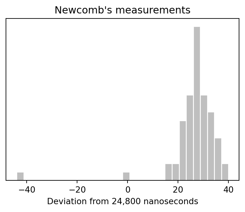
Simon Newcomb's speed-of-light measurements are recorded as deviations from 24,800 nanoseconds. The book fits a normal model with only an intercept and then checks whether replicated normal data look like the observed data. The interesting feature is the extreme low observation: a normal model centered on the bulk of the data struggles to reproduce it.
## Setup and data
```{python}
from pathlib import Path
import numpy as np
import pandas as pd
import matplotlib.pyplot as plt
from scipy import stats
import statsmodels.formula.api as smf


def ros_root():
    candidates = [
        Path("../../ROS-Examples"),
        Path("../ROS-Examples"),
        Path("/Users/alal/tmp/ros-python-book/ROS-Examples"),
    ]
    for candidate in candidates:
        if candidate.exists():
            return candidate
    return candidates[0]

root = ros_root()
newcomb = pd.read_table(root / "Newcomb/data/newcomb.txt", sep=r"\s+")
y = newcomb["y"].to_numpy()
newcomb.head()
```
```{python}
pd.Series(y).describe()
```
## Histogram of the measurements
```{python}
fig, ax = plt.subplots(figsize=(5, 3.5))
ax.hist(y, bins=30, color="0.75", edgecolor="white")
ax.set_xlabel("Deviation from 24,800 nanoseconds")
ax.set_yticks([])
ax.set_title("Newcomb's measurements")
```
## Fit the intercept-only normal model
`stan_glm(y ~ 1)` is a Gaussian model with an unknown mean and residual scale. The least-squares estimate is simply the sample mean; for posterior predictive checks we draw from the usual conjugate approximation with a noninformative prior.
```{python}
fit = smf.ols("y ~ 1", data=newcomb).fit()
fit.summary()
```
```{python}
n = len(y)
ybar = y.mean()
s2 = y.var(ddof=1)
rng = np.random.default_rng(202611)
n_sims = 4000

sigma2_draws = (n - 1) * s2 / rng.chisquare(df=n - 1, size=n_sims)
mu_draws = rng.normal(ybar, np.sqrt(sigma2_draws / n))
y_rep = rng.normal(mu_draws[:, None], np.sqrt(sigma2_draws)[:, None], size=(n_sims, n))

pd.DataFrame({
    "posterior_mean_mu": [mu_draws.mean()],
    "posterior_sd_mu": [mu_draws.std()],
    "posterior_mean_sigma": [np.sqrt(sigma2_draws).mean()],
})
```
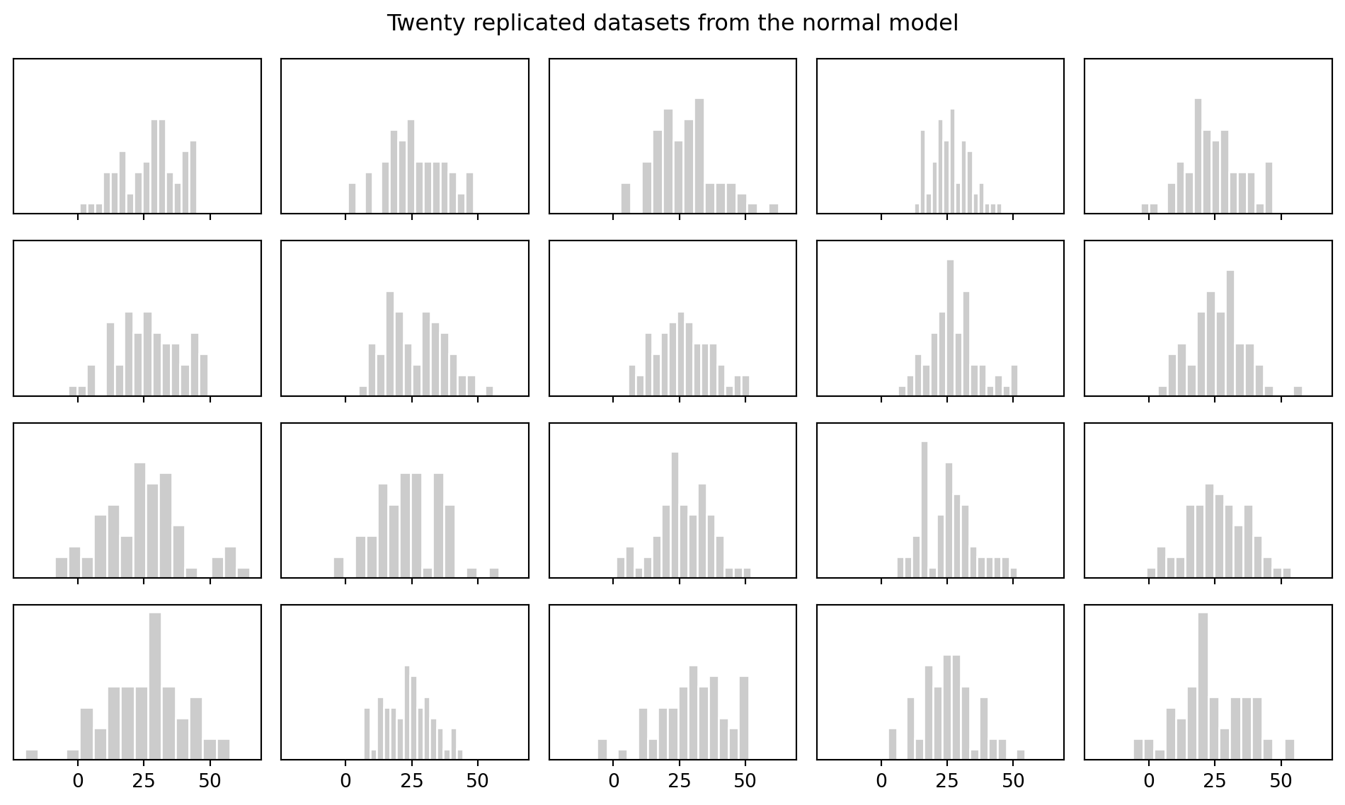
## Histograms of replicated datasets
```{python}
fig, axes = plt.subplots(4, 5, figsize=(10, 6), sharex=True, sharey=True)
for ax, s in zip(axes.ravel(), rng.choice(n_sims, size=20, replace=False)):
    ax.hist(y_rep[s], bins=15, color="0.8", edgecolor="white")
    ax.set_yticks([])
fig.suptitle("Twenty replicated datasets from the normal model")
fig.tight_layout()
```
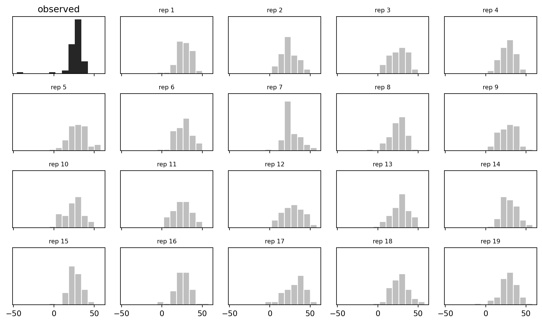
## Data histogram against predictive replications
```{python}
bins = np.arange(min(y.min(), y_rep[:19].min()) - 2, max(y.max(), y_rep[:19].max()) + 4, 8)
fig, axes = plt.subplots(4, 5, figsize=(10, 6), sharex=True, sharey=True)
axes = axes.ravel()
axes[0].hist(y, bins=bins, color="black", alpha=0.85)
axes[0].set_title("observed")
for i, ax in enumerate(axes[1:], start=1):
    ax.hist(y_rep[i - 1], bins=bins, color="0.75", edgecolor="white")
    ax.set_title(f"rep {i}", fontsize=8)
for ax in axes:
    ax.set_yticks([])
fig.tight_layout()
```
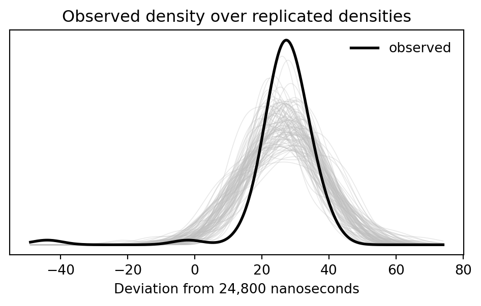
## Density overlay
```{python}
xs = np.linspace(min(y.min(), y_rep[:100].min()) - 5, max(y.max(), y_rep[:100].max()) + 5, 400)
fig, ax = plt.subplots(figsize=(6, 3))
for rep in y_rep[:100]:
    kde = stats.gaussian_kde(rep)
    ax.plot(xs, kde(xs), color="0.75", linewidth=0.6, alpha=0.35)
obs_kde = stats.gaussian_kde(y)
ax.plot(xs, obs_kde(xs), color="black", linewidth=2, label="observed")
ax.set_yticks([])
ax.set_xlabel("Deviation from 24,800 nanoseconds")
ax.set_title("Observed density over replicated densities")
ax.legend(frameon=False)
```
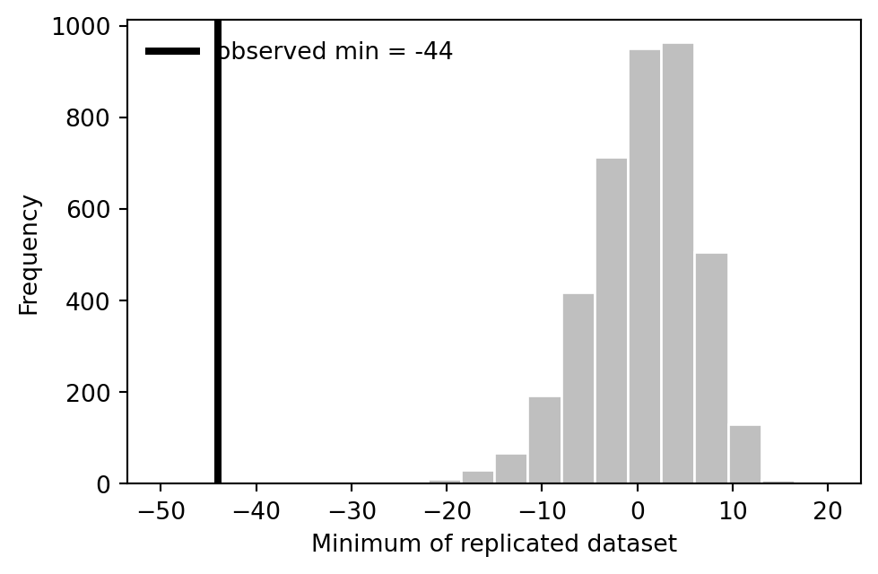
## Test statistic: the minimum
The book's posterior predictive check focuses on `min(y)`. If the observed minimum lies far in the tail of replicated minima, the normal model misses an important feature of the data.
```{python}
test_rep = y_rep.min(axis=1)
test_obs = y.min()
pp_value = np.mean(test_rep <= test_obs)
pd.DataFrame({"observed_min": [test_obs], "posterior_predictive_p_value": [pp_value]})
```
```{python}
fig, ax = plt.subplots(figsize=(5.5, 3.5))
ax.hist(test_rep, bins=20, range=(-50, 20), color="0.75", edgecolor="white")
ax.axvline(test_obs, color="black", linewidth=3, label=f"observed min = {test_obs:g}")
ax.set_xlabel("Minimum of replicated dataset")
ax.set_ylabel("Frequency")
ax.legend(frameon=False)
```
## CmdStanPy note
```{python}
#| eval: false
from cmdstanpy import CmdStanModel

# A direct Stan implementation is a one-parameter-location normal model plus
# generated quantities for y_rep and min(y_rep).  The conjugate simulation above
# is enough for the posterior predictive lesson in this example.
```