# National Election Study: logistic regression, prediction, and separation
Source: `NES/nes_logistic.Rmd`
This page ports the ROS logistic-regression example. It uses the 1992 National Election Study for a simple vote-on-income model, then repeats logistic regressions across years to show changing income effects and the instability created by separation.
## Setup and data
```{python}
from pathlib import Path
import numpy as np
import pandas as pd
import matplotlib.pyplot as plt
import statsmodels.api as sm
import statsmodels.formula.api as smf
from scipy.special import expit
from python.bayes_glm import bayes_logit

root = Path("../../ROS-Examples")
nes_dir = root / "NES"
nes = pd.read_csv(nes_dir / "data/nes.txt", sep=r"\s+", index_col=0, na_values=["NA"])
nes.head()
```
The source R page first keeps 1992 respondents with a valid Democratic or Republican presidential vote.
```{python}
ok92 = (nes["year"] == 1992) & nes["rvote"].notna() & nes["dvote"].notna() & ((nes["rvote"] == 1) | (nes["dvote"] == 1))
nes92 = nes.loc[ok92].copy()
nes92[["year", "income", "rvote", "dvote", "presvote"]].head()
```
## A single-predictor logistic regression
The R model is `stan_glm(rvote ~ income, family=binomial(link="logit"))`. For the main Bayesian port, fit the same Bernoulli-logit model with weak Normal priors using the shared lightweight helper.
```{python}
fit_1 = bayes_logit("rvote ~ income", data=nes92, draws=4000, prior_scale=2.5, seed=1992)
fit_1.summary()
```
```{python}
new = pd.DataFrame({"income": [5]})
eta_draw = fit_1.beta_draws @ np.array([1.0, 5.0])
p_draw = expit(eta_draw)

pd.DataFrame({
    "linear_predictor_mean": [eta_draw.mean()],
    "linear_predictor_sd": [eta_draw.std(ddof=1)],
    "expected_probability_mean": [p_draw.mean()],
    "expected_probability_sd": [p_draw.std(ddof=1)],
})
```
The distinction among linear predictor, expected outcome, and posterior predictive draw is clearest when using the posterior coefficient draws directly. This mirrors the operations performed by `posterior_linpred`, `posterior_epred`, and `posterior_predict` in the R example.
```{python}
rng = np.random.default_rng(1992)
draws = fit_1.beta_draws
X_new = np.column_stack([np.ones(5), np.arange(1, 6)])
linpred = draws @ X_new.T
epred = expit(linpred)
postpred = rng.binomial(1, epred)

summary_pred = pd.DataFrame(
    {
        "income": np.arange(1, 6),
        "p_mean": epred.mean(axis=0),
        "p_sd": epred.std(axis=0),
        "y_pred_mean": postpred.mean(axis=0),
    }
)
summary_pred
```
```{python}
prob_rich_gt_next = np.mean(epred[:, 4] > epred[:, 3])
diff_interval = np.quantile(epred[:, 4] - epred[:, 3], [0.025, 0.975])
prob_rich_gt_next, diff_interval
```
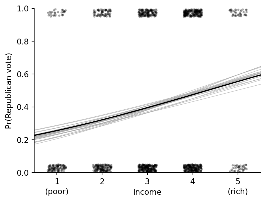
## Jittered data and fitted curve
```{python}
rng = np.random.default_rng(2141)
n = len(nes92)
income_jitt = nes92["income"].to_numpy() + rng.uniform(-0.2, 0.2, size=n)
vote_jitt = nes92["rvote"].to_numpy() + np.where(nes92["rvote"].to_numpy() == 0, rng.uniform(0.005, 0.05, size=n), rng.uniform(-0.05, -0.005, size=n))

x_grid = np.linspace(0.5, 5.5, 200)
X_grid = pd.DataFrame({"income": x_grid})

fig, ax = plt.subplots(figsize=(5.2, 3.8))
for draw in draws[rng.choice(len(draws), 25, replace=False)]:
    ax.plot(x_grid, expit(draw[0] + draw[1] * x_grid), color="0.65", lw=0.6, alpha=0.7)
ax.plot(x_grid, fit_1.epred(X_grid).mean(axis=0), color="black", lw=1.5)
ax.scatter(income_jitt, vote_jitt, s=4, color="black", alpha=0.25)
ax.set_xticks(range(1, 6))
ax.text(1, -0.13, "(poor)", ha="center", transform=ax.get_xaxis_transform())
ax.text(5, -0.13, "(rich)", ha="center", transform=ax.get_xaxis_transform())
ax.set(xlim=(0.5, 5.5), ylim=(0, 1), xlabel="Income", ylabel="Pr(Republican vote)")
ax.spines[["top", "right"]].set_visible(False)
```
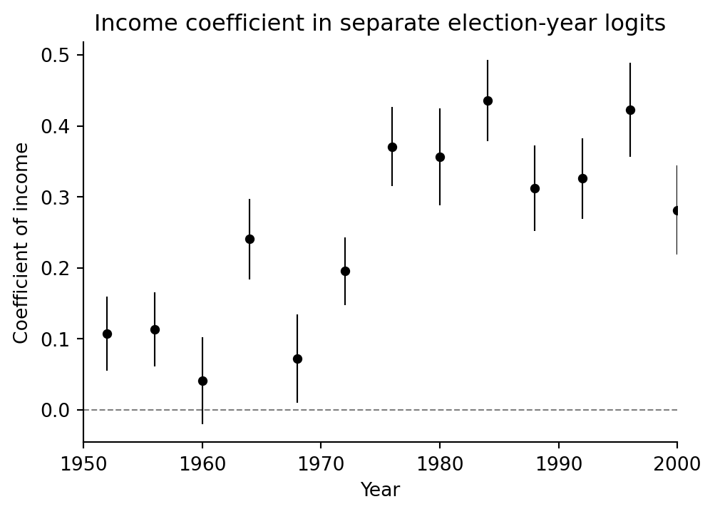
## Income coefficient by election year
```{python}
years = list(range(1952, 2001, 4))
rows = []
for year in years:
    ok = (nes["year"] == year) & nes["presvote"].notna() & (nes["presvote"] < 3) & nes["vote"].notna() & nes["income"].notna()
    d = nes.loc[ok, ["presvote", "income"]].copy()
    d["vote_rep"] = d["presvote"] - 1
    if d["vote_rep"].nunique() < 2:
        continue
    fit_y = smf.glm("vote_rep ~ income", data=d, family=sm.families.Binomial()).fit()
    rows.append({"year": year, "coef": fit_y.params["income"], "se": fit_y.bse["income"], "nobs": fit_y.nobs})

fits = pd.DataFrame(rows)
fits
```
```{python}
fig, ax = plt.subplots(figsize=(5.6, 3.8))
ax.axhline(0, color="0.5", ls="--", lw=0.8)
ax.errorbar(fits["year"], fits["coef"], yerr=fits["se"], fmt="o", color="black", ms=4, lw=0.8)
ax.set(xlim=(1950, 2000), xlabel="Year", ylabel="Coefficient of income", title="Income coefficient in separate election-year logits")
ax.spines[["top", "right"]].set_visible(False)
```
## In-sample accuracy and log score
```{python}
predp = fit_1.epred().mean(axis=0)
y = nes92["rvote"].to_numpy()
accuracy_parts = (predp[y == 1].mean(), (1 - predp[y == 0]).mean())
log_score = np.log(np.r_[predp[y == 1], 1 - predp[y == 0]]).sum()
accuracy_parts, log_score
```
A light leave-one-out calculation can be done by refitting the model after dropping each observation. This is slower than PSIS-LOO from the Stan ecosystem, but it is transparent for a simple GLM.
```{python}
def loo_log_score(data):
    values = []
    for i in data.index:
        train = data.drop(index=i)
        test = data.loc[[i]]
        fit_i = smf.glm("rvote ~ income", data=train, family=sm.families.Binomial()).fit(disp=0)
        p_i = fit_i.predict(test)[0]
        y_i = test["rvote"].iloc[0]
        values.append(np.log(p_i if y_i == 1 else 1 - p_i))
    return np.sum(values)

# loo_log_score(nes92)  # uncomment to run the exact leave-one-out refit
```
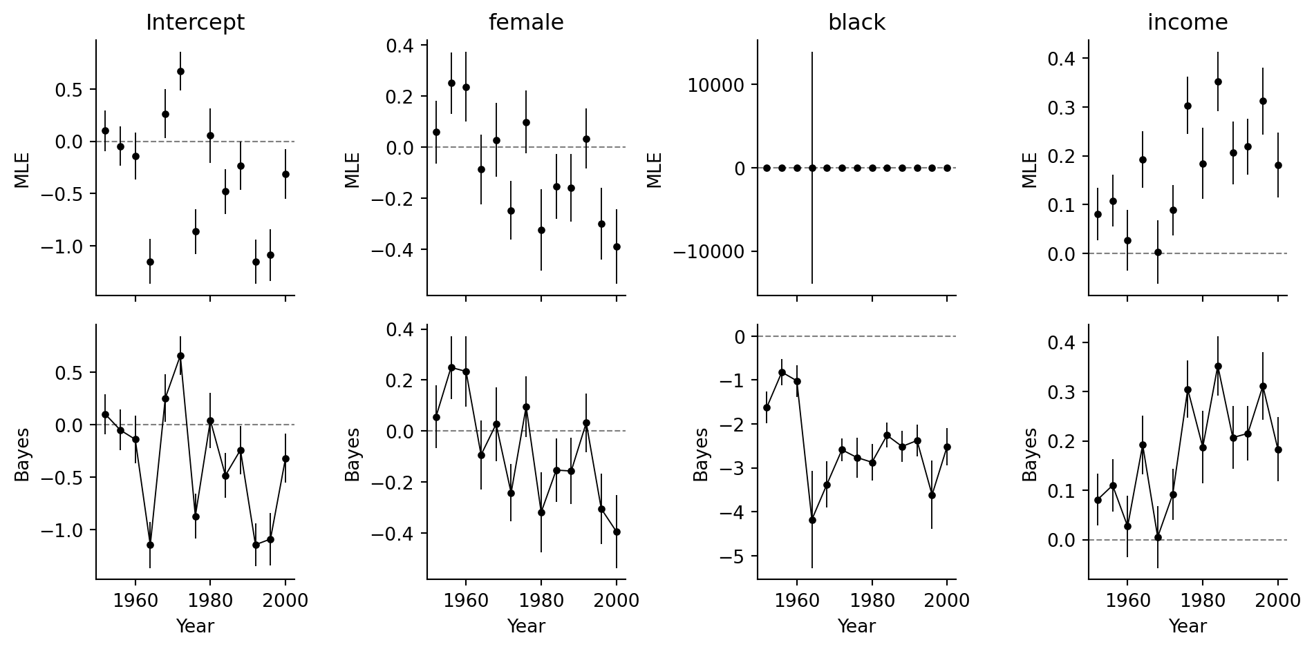
## Separation and weak regularization
The final part of the source example compares classical `glm` with `stan_glm` for `rvote ~ female + black + income`. In years with quasi-complete separation, maximum-likelihood coefficients can become huge or have enormous standard errors. A weakly regularized logistic model stabilizes the fit.
```{python}
terms = ["Intercept", "female", "black", "income"]
sep_rows = []
base = nes.loc[nes[["rvote", "female", "black", "income"]].notna().all(axis=1)].copy()

for year in years:
    d = base.loc[base["year"] == year].copy()
    if d["rvote"].nunique() < 2:
        continue
    try:
        fit_glm = smf.glm("rvote ~ female + black + income", data=d, family=sm.families.Binomial()).fit()
        for term in terms:
            sep_rows.append({"year": year, "term": term, "model": "MLE", "coef": fit_glm.params[term], "se": fit_glm.bse[term]})
    except Exception as err:
        sep_rows.append({"year": year, "term": "model", "model": "MLE", "coef": np.nan, "se": np.nan, "note": str(err)})

sep = pd.DataFrame(sep_rows)
sep.head()
```
The Bayesian fit uses the same weak Normal prior in every year. Its posterior mean and standard deviation stay finite when the likelihood alone is weakly identified.
```{python}
reg_rows = []
for year in years:
    d = base.loc[base["year"] == year].copy()
    if d["rvote"].nunique() < 2:
        continue
    fit_bayes_y = bayes_logit("rvote ~ female + black + income", data=d, draws=2000, prior_scale=2.5, seed=year)
    for term, coef, se in zip(fit_bayes_y.coef_names, fit_bayes_y.beta_draws.mean(axis=0), fit_bayes_y.beta_draws.std(axis=0, ddof=1)):
        reg_rows.append({"year": year, "term": term, "model": "Bayes normal-prior", "coef": coef, "se": se})

regularized = pd.DataFrame(reg_rows)
regularized.head()
```
```{python}
fig, axes = plt.subplots(2, 4, figsize=(10, 5), sharex=True)
for col, term in enumerate(terms):
    d_mle = sep.loc[sep["term"] == term]
    axes[0, col].axhline(0, color="0.5", ls="--", lw=0.8)
    axes[0, col].errorbar(d_mle["year"], d_mle["coef"], yerr=d_mle["se"], fmt="o", color="black", ms=3, lw=0.7)
    axes[0, col].set_title(term)
    axes[0, col].set_ylabel("MLE")

    d_reg = regularized.loc[regularized["term"] == term]
    axes[1, col].axhline(0, color="0.5", ls="--", lw=0.8)
    axes[1, col].errorbar(d_reg["year"], d_reg["coef"], yerr=d_reg["se"], fmt="o-", color="black", ms=3, lw=0.7)
    axes[1, col].set_ylabel("Bayes")
    axes[1, col].set_xlabel("Year")

for ax in axes.ravel():
    ax.set_xticks([1960, 1980, 2000])
    ax.spines[["top", "right"]].set_visible(False)
fig.tight_layout()
```
## CmdStanPy version of the single-predictor model
Use this small Stan model if exact Stan sampling is needed instead of the lightweight Laplace posterior used above.
```{python}
from cmdstanpy import CmdStanModel

stan_code = """
data {
  int<lower=1> N;
  vector[N] income;
  array[N] int<lower=0, upper=1> rvote;
}
parameters {
  real alpha;
  real beta;
}
model {
  alpha ~ normal(0, 2.5);
  beta ~ normal(0, 2.5);
  rvote ~ bernoulli_logit(alpha + beta * income);
}
"""
stan_file = Path("_generated/nes_vote_income.stan")
stan_file.parent.mkdir(exist_ok=True)
stan_file.write_text(stan_code)
model = CmdStanModel(stan_file=str(stan_file))
fit = model.sample(
    data={"N": len(nes92), "income": nes92["income"].to_numpy(), "rvote": nes92["rvote"].astype(int).to_list()},
    seed=1992,
    chains=4,
    parallel_chains=4,
    show_progress=False,
)
fit.draws_pd()[["alpha", "beta"]].describe(percentiles=[0.05, 0.5, 0.95])
```