Code
import numpy as np
import pandas as pd
import matplotlib.pyplot as plt
import statsmodels.api as sm

rng = np.random.default_rng(2141)Source: Simplest/simplest_lm.Rmd
This page ports the least-squares version of the ROS “simplest” example. The point is pedagogical: fitting a line, estimating one mean, and estimating a difference in means are all ordinary linear regressions with different design matrices.
import numpy as np
import pandas as pd
import matplotlib.pyplot as plt
import statsmodels.api as sm
rng = np.random.default_rng(2141)The R code uses x = 1:20, intercept 0.2, slope 0.3, and residual standard deviation 0.5. NumPy’s random stream is not identical to R’s, but the data-generating setup is the same.
x = np.arange(1, 21)
a = 0.2
b = 0.3
sigma = 0.5
y = a + b * x + sigma * rng.normal(size=len(x))
fake = pd.DataFrame({"x": x, "y": y})

fit = sm.OLS(fake["y"], sm.add_constant(fake["x"])).fit()
fit.summary()| Dep. Variable: | y | R-squared: | 0.920 |
|---|---|---|---|
| Model: | OLS | Adj. R-squared: | 0.916 |
| Method: | Least Squares | F-statistic: | 207.0 |
| Date: | Sun, 31 May 2026 | Prob (F-statistic): | 2.58e-11 |
| Time: | 23:05:42 | Log-Likelihood: | -14.916 |
| No. Observations: | 20 | AIC: | 33.83 |
| Df Residuals: | 18 | BIC: | 35.82 |
| Df Model: | 1 | ||
| Covariance Type: | nonrobust |
| coef | std err | t | P>|t| | [0.025 | 0.975] | |
|---|---|---|---|---|---|---|
| const | 0.2513 | 0.250 | 1.006 | 0.328 | -0.273 | 0.776 |
| x | 0.3000 | 0.021 | 14.388 | 0.000 | 0.256 | 0.344 |
| Omnibus: | 0.393 | Durbin-Watson: | 1.430 |
|---|---|---|---|
| Prob(Omnibus): | 0.822 | Jarque-Bera (JB): | 0.528 |
| Skew: | 0.230 | Prob(JB): | 0.768 |
| Kurtosis: | 2.350 | Cond. No. | 25.0 |
a_hat, b_hat = fit.params["const"], fit.params["x"]
x_bar = fake["x"].mean()

fig, ax = plt.subplots(figsize=(6, 4.4))
ax.scatter(fake["x"], fake["y"], color="black", s=25)
ax.plot(fake["x"], a_hat + b_hat * fake["x"], color="black")
ax.text(x_bar, a_hat + b_hat * x_bar, f"   y = {a_hat:.2f} + {b_hat:.2f} x", va="center")
ax.set(title="Data and fitted regression line", xlabel="x", ylabel="y")
ax.spines[["top", "right"]].set_visible(False)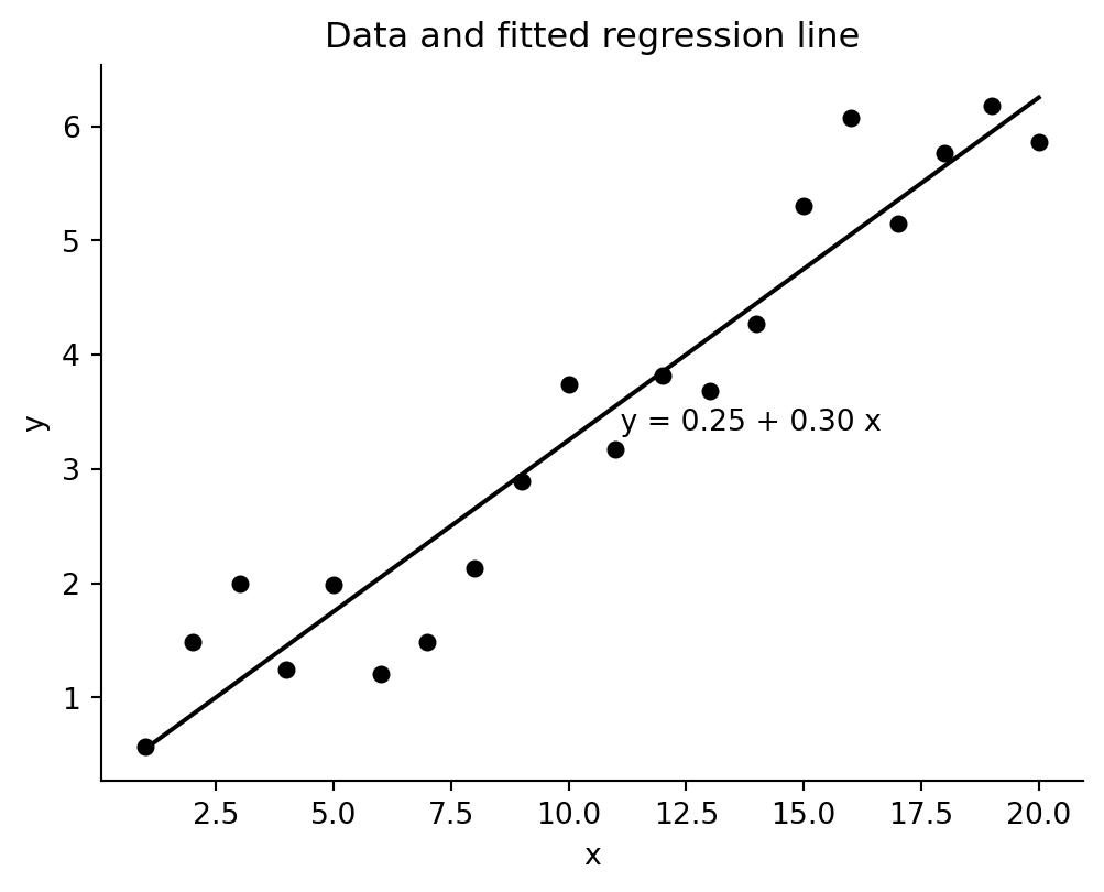
A regression on only a constant estimates the sample mean. Its standard error is the same as the usual standard error of the mean.
rng = np.random.default_rng(2141)
n_0 = 20
y_0 = np.round(rng.normal(2, 5, size=n_0), 1)

mean_direct = y_0.mean()
se_direct = y_0.std(ddof=1) / np.sqrt(n_0)
fit_mean = sm.OLS(y_0, np.ones((n_0, 1))).fit()

pd.DataFrame(
    {
        "direct_mean": [mean_direct],
        "regression_intercept": [fit_mean.params[0]],
        "direct_se": [se_direct],
        "regression_se": [fit_mean.bse[0]],
    }
)| direct_mean | regression_intercept | direct_se | regression_se | |
|---|---|---|---|---|
| 0 | 2.515 | 2.515 | 1.171465 | 1.171465 |
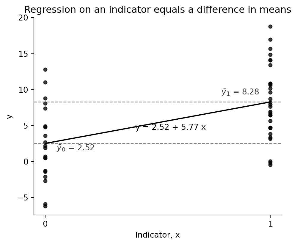
Now simulate a second group. The slope on an indicator variable is exactly the difference between the two group means.
rng = np.random.default_rng(2141)
n_1 = 30
y_1 = rng.normal(8, 5, size=n_1)

diff = y_1.mean() - y_0.mean()
se_0 = y_0.std(ddof=1) / np.sqrt(n_0)
se_1 = y_1.std(ddof=1) / np.sqrt(n_1)
se_diff = np.sqrt(se_0**2 + se_1**2)

y_all = np.r_[y_0, y_1]
group = np.r_[np.zeros(n_0), np.ones(n_1)]
fit_diff = sm.OLS(y_all, sm.add_constant(group)).fit()

pd.DataFrame(
    {
        "difference_in_means": [diff],
        "regression_slope": [fit_diff.params[1]],
        "two_sample_se": [se_diff],
        "ols_slope_se": [fit_diff.bse[1]],
    }
)| difference_in_means | regression_slope | two_sample_se | ols_slope_se | |
|---|---|---|---|---|
| 0 | 5.767634 | 5.767634 | 1.492224 | 1.481843 |
The standard errors differ slightly because the classical OLS regression uses a pooled residual variance, whereas the direct calculation above allows different variances in the two groups. The coefficient identity itself is exact.
fig, ax = plt.subplots(figsize=(5.6, 4.5))
ax.scatter(group, y_all, color="black", s=18, alpha=0.75)
ax.set_xticks([0, 1])
ax.set(xlabel="Indicator, x", ylabel="y", title="Regression on an indicator equals a difference in means")
ax.axhline(y_0.mean(), color="0.5", ls="--", lw=1)
ax.axhline(y_1.mean(), color="0.5", ls="--", lw=1)
xx = np.array([0, 1])
ax.plot(xx, fit_diff.params[0] + fit_diff.params[1] * xx, color="black")
ax.text(0.05, y_0.mean() - 1, rf"$\bar y_0$ = {y_0.mean():.2f}", color="0.25")
ax.text(0.95, y_1.mean() + 1, rf"$\bar y_1$ = {y_1.mean():.2f}", color="0.25", ha="right")
ax.text(0.4, fit_diff.params[0] + 0.5 * fit_diff.params[1] - 1, f"y = {fit_diff.params[0]:.2f} + {fit_diff.params[1]:.2f} x")
ax.spines[["top", "right"]].set_visible(False)