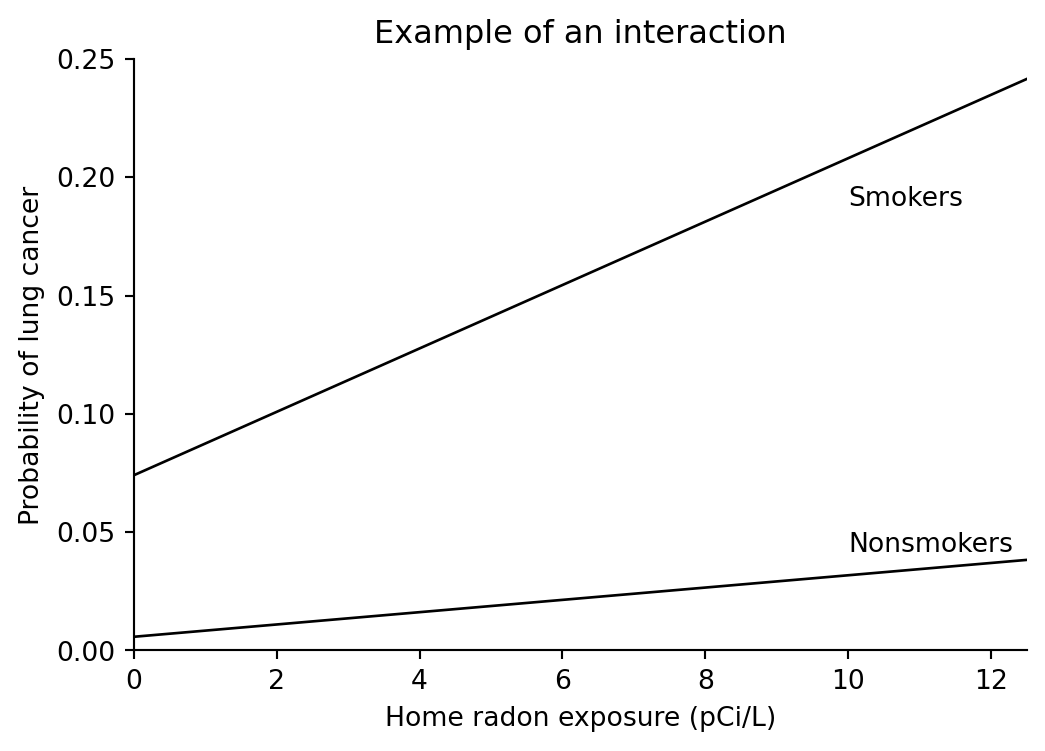
The original page is a small plotting example from Chapter 1: two straight-line risk curves whose slopes differ by smoking status. The point is the visual meaning of an interaction: the effect of home radon exposure is larger for smokers than for nonsmokers.
Plot the two interaction lines
Code
import numpy as npimport pandas as pdimport matplotlib.pyplot as pltradon = np.linspace(0, 12.5, 200)curves = pd.DataFrame({"radon": np.tile(radon, 2),"smoking": np.repeat(["Smokers", "Nonsmokers"], len(radon)),})curves["prob_lung_cancer"] = np.where( curves["smoking"].eq("Smokers"),0.07409+0.0134* curves["radon"],0.00579+0.0026* curves["radon"],)fig, ax = plt.subplots(figsize=(6, 4))for label, grp in curves.groupby("smoking"): ax.plot(grp["radon"], grp["prob_lung_cancer"], color="black", lw=1)ax.text(10, 0.07409+10*0.0134-0.02, "Smokers")ax.text(10, 0.00579+10*0.0026+0.01, "Nonsmokers")ax.set( xlim=(0, 12.5), ylim=(0, 0.25), xlabel="Home radon exposure (pCi/L)", ylabel="Probability of lung cancer", title="Example of an interaction",)ax.spines[["top", "right"]].set_visible(False)
Regression form
A linear interaction model for these two lines can be written as
[ () = + x + S + xS, ]
where x is radon exposure and S=1 for smokers. Taking nonsmokers as the baseline gives:
The interaction coefficient is the difference in slopes. In this stylized example, each additional pCi/L of radon changes the probability by 0.0026 for nonsmokers and by 0.0134 for smokers.
Source Code
# Interactions: radon and smokingSource: `Interactions/interactions.Rmd`The original page is a small plotting example from Chapter 1: two straight-line risk curves whose slopes differ by smoking status. The point is the visual meaning of an interaction: the effect of home radon exposure is larger for smokers than for nonsmokers.## Plot the two interaction lines```{python}import numpy as npimport pandas as pdimport matplotlib.pyplot as pltradon = np.linspace(0, 12.5, 200)curves = pd.DataFrame({"radon": np.tile(radon, 2),"smoking": np.repeat(["Smokers", "Nonsmokers"], len(radon)),})curves["prob_lung_cancer"] = np.where( curves["smoking"].eq("Smokers"),0.07409+0.0134* curves["radon"],0.00579+0.0026* curves["radon"],)fig, ax = plt.subplots(figsize=(6, 4))for label, grp in curves.groupby("smoking"): ax.plot(grp["radon"], grp["prob_lung_cancer"], color="black", lw=1)ax.text(10, 0.07409+10*0.0134-0.02, "Smokers")ax.text(10, 0.00579+10*0.0026+0.01, "Nonsmokers")ax.set( xlim=(0, 12.5), ylim=(0, 0.25), xlabel="Home radon exposure (pCi/L)", ylabel="Probability of lung cancer", title="Example of an interaction",)ax.spines[["top", "right"]].set_visible(False)```## Regression formA linear interaction model for these two lines can be written as\[\Pr(\text{lung cancer}) = \alpha + \beta x + \gamma S + \delta xS,\]where `x` is radon exposure and `S=1` for smokers. Taking nonsmokers as the baseline gives:```{python}alpha =0.00579beta =0.0026gamma =0.07409-0.00579delta =0.0134-0.0026pd.Series({"Intercept": alpha, "radon": beta, "smoker": gamma, "radon:smoker": delta})```The interaction coefficient is the difference in slopes. In this stylized example, each additional pCi/L of radon changes the probability by 0.0026 for nonsmokers and by 0.0134 for smokers.