Beauty and sex ratio: when an informative prior matters

Source: SexRatio/sexratio.Rmd

This tiny example is intentionally prior-sensitive: five noisy points suggest a steep positive slope, but background knowledge says such an effect should be small. The page shows least squares, conjugate normal shrinkage for a slope, and the corresponding Bayesian regression setup.

Code

import numpy as np
import pandas as pd
import matplotlib.pyplot as plt
import statsmodels.formula.api as smf

Data

Code

x = np.arange(-2, 3)
y = np.array([50, 44, 50, 47, 56])
sexratio = pd.DataFrame({"x": x, "y": y})
sexratio

	x	y
0	-2	50
1	-1	44
2	0	50
3	1	47
4	2	56

Least-squares regression

Code

fit = smf.ols("y ~ x", data=sexratio).fit()
pd.DataFrame({"estimate": fit.params, "std_error": fit.bse})

	estimate	std_error
Intercept	49.4	1.944222
x	1.5	1.374773

Code

fig, axs = plt.subplots(1, 2, figsize=(9, 3), sharey=True)
axs[0].scatter(x, y, color="black")
axs[0].set_title("data")
axs[1].scatter(x, y, color="black")
xs = np.linspace(-2, 2, 100)
axs[1].plot(xs, fit.params["Intercept"] + fit.params["x"]*xs)
axs[1].set_title("least-squares fit")
for ax in axs:
    ax.set_xlabel("parent attractiveness")
    ax.set_ylabel("% girl babies")
    ax.set_ylim(43, 57)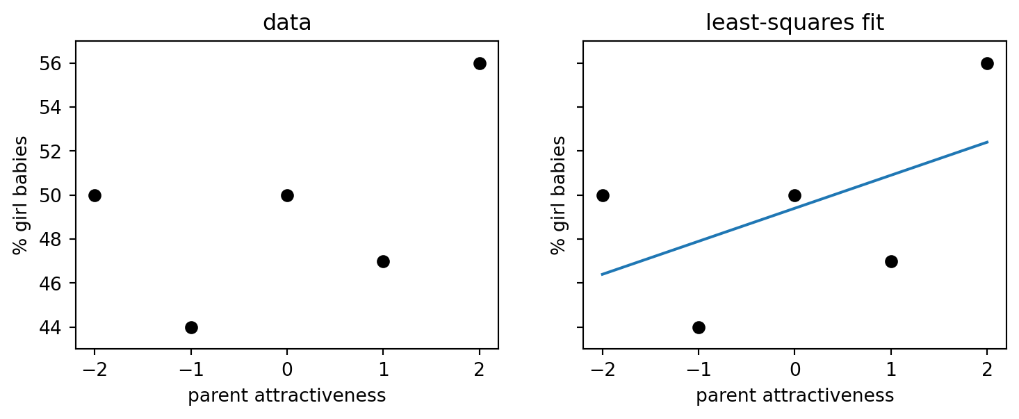

Normal-normal shrinkage calculation

The R example summarizes the conflict as theta_data = 8 with se_data = 3, against a prior centered at 0 with standard error 0.25.

Code

theta_prior, se_prior = 0.0, 0.25
theta_data, se_data = 8.0, 3.0
precision_post = 1/se_prior**2 + 1/se_data**2
theta_post = (theta_prior/se_prior**2 + theta_data/se_data**2) / precision_post
se_post = np.sqrt(1 / precision_post)
theta_post, se_post

(0.05517241379310345, np.float64(0.2491364395612199))

The posterior is almost identical to the prior because the data estimate is much noisier than the prior information.

Bayesian regression skeleton

data { int<lower=1> N; vector[N] x; vector[N] y; }
parameters { real alpha; real beta; real<lower=0> sigma; }
model {
  alpha ~ normal(48.8, 0.5);
  beta ~ normal(0, 0.2);
  sigma ~ exponential(1);
  y ~ normal(alpha + beta * x, sigma);
}

Code

# CmdStanPy would sample this model directly; the key modeling move is the informative prior:
# beta ~ normal(0, 0.2), alpha ~ normal(48.8, 0.5)