# Roaches
Source: `Roaches/roaches.Rmd`
This example analyzes an integrated pest-management experiment in urban apartments. The response `y` is the post-treatment roach count. Predictors include the baseline roach count, treatment assignment, senior-building indicator, and an exposure offset. The original R page compares negative-binomial, Poisson, and zero-inflated negative-binomial models using `rstanarm`, `brms`, and posterior predictive checks.
## Setup and data
```{python}
from pathlib import Path
import numpy as np
import pandas as pd
import matplotlib.pyplot as plt
import statsmodels.api as sm
import statsmodels.formula.api as smf
from scipy.stats import gaussian_kde

root = Path("../../ROS-Examples")
roaches = pd.read_csv(root / "Roaches/data/roaches.csv", index_col=0)
roaches["roach100"] = roaches["roach1"] / 100
roaches["logp1_roach1"] = np.log1p(roaches["roach1"])
roaches["log_exposure2"] = np.log(roaches["exposure2"])
roaches.head()
```
```{python}
roaches.describe()
```
## Negative-binomial model
The R original fits:
```r
stan_glm(y ~ roach100 + treatment + senior,
         family=neg_binomial_2,
         offset=log(exposure2), data=roaches)
```
A close maximum-likelihood analogue is `statsmodels.discrete.NegativeBinomial`, with the offset supplied explicitly.
```{python}
nb_model = sm.NegativeBinomial.from_formula(
    "y ~ roach100 + treatment + senior",
    data=roaches,
    offset=roaches["log_exposure2"],
)
fit_1 = nb_model.fit(disp=False)
fit_1.summary()
```
```{python}
alpha_hat = fit_1.params.get("alpha", np.nan)
phi_hat = 1 / alpha_hat if alpha_hat > 0 else np.inf
pd.Series({"alpha": alpha_hat, "phi=1/alpha": phi_hat})
```
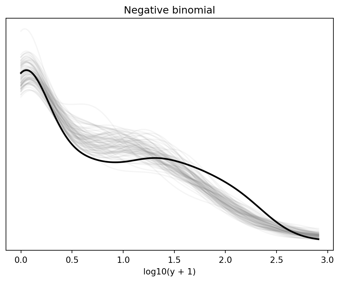
## Posterior-predictive-style checks
Without MCMC draws, we can still do the same kind of model criticism using parametric simulation at the fitted MLE. For a negative-binomial 2 model, variance is `mu + alpha * mu^2`, equivalently `phi = 1 / alpha`.
```{python}
rng = np.random.default_rng(3579)

X = fit_1.model.exog
beta = fit_1.params.drop("alpha").to_numpy()
mu_nb = np.exp(X @ beta + roaches["log_exposure2"].to_numpy())
alpha = fit_1.params["alpha"]
phi = 1 / alpha
p = phi / (phi + mu_nb)
yrep_1 = rng.negative_binomial(phi, p, size=(400, len(roaches)))

def check_stats(y, yrep):
    return pd.DataFrame({
        "observed": [np.mean(y == 0), np.mean(y == 1), np.quantile(y, 0.95), np.quantile(y, 0.99), np.max(y)],
        "rep_mean": [np.mean(yrep == 0), np.mean(yrep == 1), np.mean(np.quantile(yrep, 0.95, axis=1)), np.mean(np.quantile(yrep, 0.99, axis=1)), np.mean(np.max(yrep, axis=1))],
    }, index=["Pr(y=0)", "Pr(y=1)", "q95", "q99", "max"])

check_stats(roaches.y.to_numpy(), yrep_1)
```
```{python}
def density_overlay(ax, observed, replicated, title):
    grid = np.linspace(0, max(np.max(observed), np.percentile(replicated, 99)), 250)
    for draw in replicated[:80]:
        ax.plot(grid, gaussian_kde(draw)(grid), color="gray", alpha=0.08)
    ax.plot(grid, gaussian_kde(observed)(grid), color="black", linewidth=2)
    ax.set_title(title)
    ax.set_xlabel("log10(y + 1)")
    ax.set_yticks([])

fig, ax = plt.subplots()
density_overlay(ax, np.log10(roaches.y + 1), np.log10(yrep_1 + 1), "Negative binomial")
```
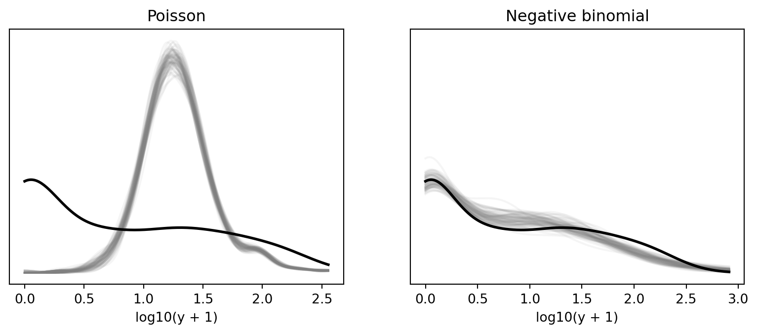
## Poisson model
Poisson regression is a restricted version of the count model in which variance equals the mean.
```{python}
fit_2 = smf.glm(
    "y ~ roach100 + treatment + senior",
    data=roaches,
    family=sm.families.Poisson(),
    offset=roaches["log_exposure2"],
).fit()
fit_2.summary()
```
```{python}
mu_pois = fit_2.predict(roaches, offset=roaches["log_exposure2"])
yrep_2 = rng.poisson(mu_pois, size=(400, len(roaches)))

pd.concat(
    {
        "negative_binomial": check_stats(roaches.y.to_numpy(), yrep_1)["rep_mean"],
        "poisson": check_stats(roaches.y.to_numpy(), yrep_2)["rep_mean"],
        "observed": check_stats(roaches.y.to_numpy(), yrep_2)["observed"],
    },
    axis=1,
)
```
```{python}
fig, axes = plt.subplots(1, 2, figsize=(10, 3.5), sharey=True)
density_overlay(axes[0], np.log10(roaches.y + 1), np.log10(yrep_2 + 1), "Poisson")
density_overlay(axes[1], np.log10(roaches.y + 1), np.log10(yrep_1 + 1), "Negative binomial")
```
```{python}
pd.Series({
    "nb_aic": fit_1.aic,
    "poisson_aic": fit_2.aic,
    "poisson_pearson_dispersion": fit_2.pearson_chi2 / fit_2.df_resid,
})
```
The Poisson model typically underestimates the number of zeros and the extreme upper tail; the negative-binomial model's extra dispersion helps.
## Zero-inflated negative binomial
The R page switches to `brms` for a zero-inflated negative-binomial model. `statsmodels` has a frequentist zero-inflated negative-binomial implementation. We use the same covariates in both the count and inflation components.
```{python}
from statsmodels.discrete.count_model import ZeroInflatedNegativeBinomialP

exog = sm.add_constant(roaches[["logp1_roach1", "treatment", "senior"]])
zinb_model = ZeroInflatedNegativeBinomialP(
    endog=roaches["y"],
    exog=exog,
    exog_infl=exog,
    offset=roaches["log_exposure2"],
    inflation="logit",
)
try:
    fit_3 = zinb_model.fit(method="bfgs", maxiter=200, disp=False)
    zinb_summary = fit_3.summary()
except Exception as err:
    fit_3 = None
    zinb_summary = f"Zero-inflated NB fit did not converge in this environment: {err}"
zinb_summary
```
```{python}
pd.Series({
    "negative_binomial_aic": fit_1.aic,
    "poisson_aic": fit_2.aic,
    "zero_inflated_nb_aic": np.nan if fit_3 is None else fit_3.aic,
})
```
`ZeroInflatedNegativeBinomialP` prediction APIs and optimizers vary across `statsmodels` versions, so for a robust page we use the fitted summary/AIC when available rather than requiring replicated zero-inflated draws in evaluated code.
## CmdStanPy negative-binomial model
```{python}
#| eval: false
from cmdstanpy import CmdStanModel

stan_code = """
data {
  int<lower=1> N;
  vector[N] roach100;
  vector[N] treatment;
  vector[N] senior;
  vector[N] log_exposure;
  array[N] int<lower=0> y;
}
parameters {
  real alpha;
  real beta_roach;
  real beta_treatment;
  real beta_senior;
  real<lower=0> phi;
}
model {
  alpha ~ normal(0, 5);
  beta_roach ~ normal(0, 2);
  beta_treatment ~ normal(0, 2);
  beta_senior ~ normal(0, 2);
  phi ~ exponential(1);
  y ~ neg_binomial_2_log(
    alpha + beta_roach * roach100 + beta_treatment * treatment + beta_senior * senior + log_exposure,
    phi
  );
}
generated quantities {
  array[N] int y_rep;
  for (n in 1:N) {
    real eta = alpha + beta_roach * roach100[n] + beta_treatment * treatment[n] + beta_senior * senior[n] + log_exposure[n];
    y_rep[n] = neg_binomial_2_log_rng(eta, phi);
  }
}
"""
Path("roaches_nb.stan").write_text(stan_code)
model = CmdStanModel(stan_file="roaches_nb.stan")
fit = model.sample(
    data={
        "N": len(roaches),
        "roach100": roaches.roach100.to_numpy(),
        "treatment": roaches.treatment.to_numpy(),
        "senior": roaches.senior.to_numpy(),
        "log_exposure": roaches.log_exposure2.to_numpy(),
        "y": roaches.y.astype(int).to_numpy(),
    },
    seed=3579,
)
fit.summary().loc[["alpha", "beta_roach", "beta_treatment", "beta_senior", "phi"]]
```
## CmdStanPy zero-inflated negative-binomial sketch
Stan can also express the `brms` model directly by adding a logit model for structural zeros. This chunk is a template because the full model is slower and more fragile than the negative-binomial baseline.
```{python}
#| eval: false
zinb_stan_code = """
// In the model block, for each observation n:
// if (y[n] == 0)
//   target += log_sum_exp(
//     bernoulli_logit_lpmf(1 | zi_eta[n]),
//     bernoulli_logit_lpmf(0 | zi_eta[n]) + neg_binomial_2_log_lpmf(0 | count_eta[n], phi)
//   );
// else
//   target += bernoulli_logit_lpmf(0 | zi_eta[n]) + neg_binomial_2_log_lpmf(y[n] | count_eta[n], phi);
"""
```