Code
import numpy as np
import pandas as pd
import matplotlib.pyplot as plt
import statsmodels.formula.api as smf

rng = np.random.default_rng(2243)Source: FakeMidtermFinal/simulation.Rmd
This example simulates 1,000 students with a latent ability, a noisy midterm, and a noisy final exam. Regressing final on midterm illustrates regression toward the mean: the fitted slope is positive but well below one because the midterm score is measured with noise.
import numpy as np
import pandas as pd
import matplotlib.pyplot as plt
import statsmodels.formula.api as smf
rng = np.random.default_rng(2243)n = 1_000
true_ability = rng.normal(50, 10, size=n)
noise_1 = rng.normal(0, 10, size=n)
noise_2 = rng.normal(0, 10, size=n)
midterm = true_ability + noise_1
final = true_ability + noise_2
exams = pd.DataFrame({"midterm": midterm, "final": final})
exams.describe().round(2)| midterm | final | |
|---|---|---|
| count | 1000.00 | 1000.00 |
| mean | 50.14 | 49.96 |
| std | 14.46 | 13.66 |
| min | -0.47 | 5.63 |
| 25% | 40.04 | 41.09 |
| 50% | 50.07 | 49.96 |
| 75% | 60.05 | 58.67 |
| max | 99.69 | 94.62 |
The R version fits stan_glm(final ~ midterm). Here OLS gives the corresponding Gaussian regression estimate and standard error.
fit_1 = smf.ols("final ~ midterm", data=exams).fit()
fit_1.summary().tables[1]| coef | std err | t | P>|t| | [0.025 | 0.975] | |
|---|---|---|---|---|---|---|
| Intercept | 27.0564 | 1.365 | 19.816 | 0.000 | 24.377 | 29.736 |
| midterm | 0.4567 | 0.026 | 17.457 | 0.000 | 0.405 | 0.508 |
fit_line = pd.DataFrame({"midterm": np.linspace(0, 100, 101)})
fit_line["final_hat"] = fit_1.predict(fit_line)
fit_1.params
Intercept 27.056355
midterm 0.456750
dtype: float64fig, ax = plt.subplots(figsize=(5, 5))
ax.scatter(exams["midterm"], exams["final"], s=12, alpha=0.45, linewidths=0)
ax.plot(fit_line["midterm"], fit_line["final_hat"], color="black", linewidth=2, label="OLS fit")
for v in np.arange(0, 101, 20):
ax.axhline(v, color="0.85", linestyle="--", linewidth=0.8, zorder=0)
ax.axvline(v, color="0.85", linestyle="--", linewidth=0.8, zorder=0)
ax.set_xlim(0, 100)
ax.set_ylim(0, 100)
ax.set_xlabel("Midterm exam score")
ax.set_ylabel("Final exam score")
ax.set_aspect("equal", adjustable="box")
ax.legend(frameon=False)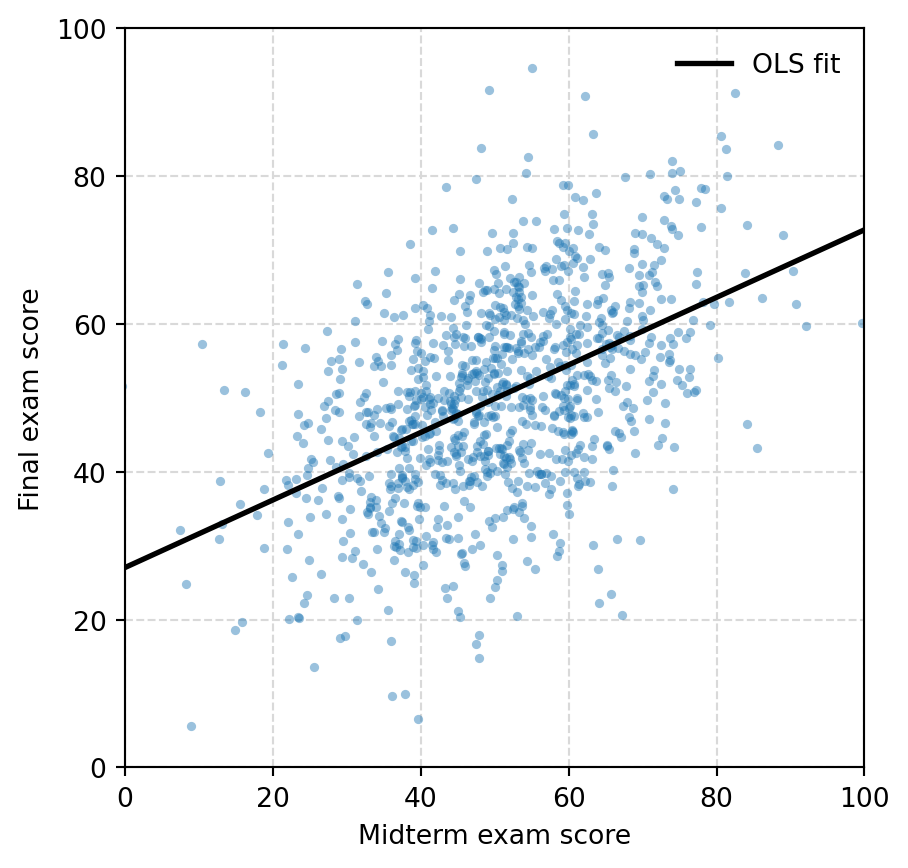
The data-generating model has equal variances for ability, midterm noise, and final noise. The population slope of final on midterm is
[ = = 0.5. ]
theoretical_slope = 10**2 / (10**2 + 10**2)
observed_corr = exams.corr().loc["midterm", "final"]
pd.Series({
    "theoretical slope": theoretical_slope,
    "estimated slope": fit_1.params["midterm"],
    "correlation": observed_corr,
}).round(3)
theoretical slope 0.500
estimated slope 0.457
correlation 0.484
dtype: float64A student with an unusually high midterm score is probably above average, but part of that high score is also positive noise. The model therefore predicts a final score closer to the population mean than the midterm score itself.