# KidIQ Bayes-R2 and LOO-R2
Source: `KidIQ/kidiq_R2.Rmd`
This page ports the `rstanarm`/`loo` example to Python. We use `statsmodels` for quick classical fits and CmdStanPy for Bayesian Gaussian regressions with pointwise log likelihoods. ArviZ supplies PSIS-LOO diagnostics analogous to the R `loo` package.
## Setup and data
```{python}
from pathlib import Path
import numpy as np
import pandas as pd
import matplotlib.pyplot as plt
import statsmodels.formula.api as smf
import patsy

root = Path("../../ROS-Examples")
kidiq = pd.read_csv(root / "KidIQ/data/kidiq.csv")
SEED = 1507
kidiq.head()
```
## Classical fits for orientation
```{python}
ols_1 = smf.ols("kid_score ~ mom_hs", data=kidiq).fit()
ols_3 = smf.ols("kid_score ~ mom_hs + mom_iq", data=kidiq).fit()
print(round(ols_1.rsquared, 3), round(ols_3.rsquared, 3))
```
## A reusable CmdStanPy Gaussian regression
The following Stan program is a direct replacement for the normal linear models fit by `rstanarm::stan_glm` in this example. It also records `log_lik[n]` for PSIS-LOO.
```{python}
from cmdstanpy import CmdStanModel
import arviz as az

stan_dir = Path("_generated_stan")
stan_dir.mkdir(exist_ok=True)
stan_file = stan_dir / "kid_iq_gaussian_lm.stan"
stan_file.write_text(r'''
data {
  int<lower=1> N;
  int<lower=1> K;
  matrix[N, K] X;
  vector[N] y;
}
parameters {
  vector[K] beta;
  real<lower=0> sigma;
}
model {
  beta ~ normal(0, 20);
  sigma ~ exponential(1.0 / 30);
  y ~ normal(X * beta, sigma);
}
generated quantities {
  vector[N] log_lik;
  vector[N] mu;
  mu = X * beta;
  for (n in 1:N) log_lik[n] = normal_lpdf(y[n] | mu[n], sigma);
}
''')

lm_model = CmdStanModel(stan_file=str(stan_file))

def design(formula, data):
    y, X = patsy.dmatrices(formula, data, return_type="dataframe")
    return np.asarray(y).ravel(), X

def sample_lm(formula, data, seed=SEED):
    y, X = design(formula, data)
    fit = lm_model.sample(
        data={"N": len(y), "K": X.shape[1], "X": X.to_numpy(), "y": y},
        seed=seed, chains=4, parallel_chains=4, show_progress=False,
    )
    return fit, X, y

fit_1, X_1, y = sample_lm("kid_score ~ mom_hs", kidiq)
fit_3, X_3, _ = sample_lm("kid_score ~ mom_hs + mom_iq", kidiq)
```
## LOO comparison
```{python}
idata_1 = az.from_cmdstanpy(posterior=fit_1, log_likelihood="log_lik")
idata_3 = az.from_cmdstanpy(posterior=fit_3, log_likelihood="log_lik")
loo_1 = az.loo(idata_1)
loo_3 = az.loo(idata_3)
az.compare({"mom_hs": idata_1, "mom_hs + mom_iq": idata_3}, ic="loo")
```
The expected log predictive density improves substantially when mother's IQ is added to the model.
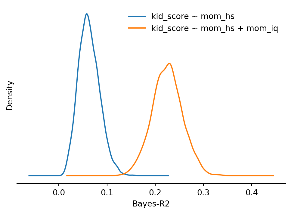
## Bayes-R2
Gelman et al.'s Bayesian R2 is computed draw by draw as
\[
R^2 = \frac{\operatorname{Var}_n(\mu_n)}{\operatorname{Var}_n(\mu_n) + \sigma^2}.
\]
```{python}
def draws_matrix(fit, X):
    draws = fit.draws_pd()
    beta_cols = [f"beta[{i}]" for i in range(1, X.shape[1] + 1)]
    beta = draws[beta_cols].to_numpy()
    sigma = draws["sigma"].to_numpy()
    mu = beta @ X.to_numpy().T
    return mu, sigma

def bayes_r2(fit, X):
    mu, sigma = draws_matrix(fit, X)
    var_fit = np.var(mu, axis=1, ddof=1)
    return var_fit / (var_fit + sigma**2)

br2_1 = bayes_r2(fit_1, X_1)
br2_3 = bayes_r2(fit_3, X_3)
round(np.median(br2_1), 3), round(np.median(br2_3), 3)
```
```{python}
fig, ax = plt.subplots(figsize=(6, 4))
for vals, label in [(br2_1, "kid_score ~ mom_hs"), (br2_3, "kid_score ~ mom_hs + mom_iq")]:
    pd.Series(vals).plot.kde(ax=ax, label=label)
ax.set(xlabel="Bayes-R2", yticks=[])
ax.legend(frameon=False)
ax.spines[["top", "right", "left"]].set_visible(False)
```
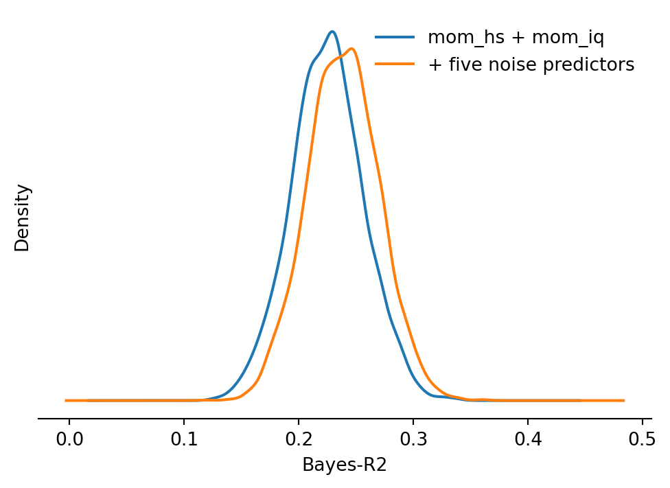
## Add five pure-noise predictors
```{python}
rng = np.random.default_rng(SEED)
kidiqr = kidiq.copy()
for j in range(1, 6):
    kidiqr[f"noise{j}"] = rng.normal(size=len(kidiqr))

noise_terms = " + ".join([f"noise{j}" for j in range(1, 6)])
fit_3n, X_3n, _ = sample_lm(f"kid_score ~ mom_hs + mom_iq + {noise_terms}", kidiqr, seed=SEED + 1)
fit_4, X_4, _ = sample_lm("kid_score ~ mom_hs + mom_iq + mom_iq:mom_hs", kidiq, seed=SEED + 2)

br2_3n = bayes_r2(fit_3n, X_3n)
br2_4 = bayes_r2(fit_4, X_4)
round(np.median(br2_3), 3), round(np.median(br2_3n), 3), round(np.median(br2_4), 3)
```
```{python}
fig, ax = plt.subplots(figsize=(6, 4))
for vals, label in [(br2_3, "mom_hs + mom_iq"), (br2_3n, "+ five noise predictors")]:
    pd.Series(vals).plot.kde(ax=ax, label=label)
ax.set(xlabel="Bayes-R2", yticks=[])
ax.legend(frameon=False)
ax.spines[["top", "right", "left"]].set_visible(False)
```
The in-sample Bayesian R2 can increase slightly after adding noise variables, because the fitted mean has more degrees of freedom. The important check is predictive performance.
## LOO-R2-style predictive comparison
The R page reports `loo_R2`. Python's ArviZ directly gives PSIS-LOO expected log predictive density; below we also compute a simple draw-wise predictive R2 from posterior fitted means to show the same qualitative story.
```{python}
idata_3n = az.from_cmdstanpy(posterior=fit_3n, log_likelihood="log_lik")
idata_4 = az.from_cmdstanpy(posterior=fit_4, log_likelihood="log_lik")
az.compare({"mom_hs + mom_iq": idata_3, "+ noise": idata_3n, "+ interaction": idata_4}, ic="loo")
```
```{python}
def posterior_predictive_r2(fit, X, y):
    mu, sigma = draws_matrix(fit, X)
    # Draw one predictive replicate for each posterior draw.
    rng = np.random.default_rng(SEED)
    y_rep = rng.normal(mu, sigma[:, None])
    residual_var = np.var(y[None, :] - y_rep, axis=1, ddof=1)
    y_var = np.var(y)
    return 1 - residual_var / y_var

for name, fit, X in [("mom_hs", fit_1, X_1), ("mom_hs + mom_iq", fit_3, X_3), ("+ noise", fit_3n, X_3n), ("+ interaction", fit_4, X_4)]:
    print(name, round(np.median(posterior_predictive_r2(fit, X, y)), 3))
```
## BlackJAX log-density sketch
For a hand-written NUTS implementation, this is the Gaussian regression target for fixed design matrix `X_3`.
```{python}
from scipy.stats import norm

X_np = X_3.to_numpy()
y_np = np.asarray(y)

def kid_iq_logdensity(params):
    beta = np.asarray(params["beta"])
    log_sigma = params["log_sigma"]
    sigma = np.exp(log_sigma)
    mu = X_np @ beta
    ll = np.sum(norm.logpdf(y_np, mu, sigma))
    prior = np.sum(norm.logpdf(beta, 0, 20)) + np.log(1 / 30) - sigma / 30 + log_sigma
    return ll + prior

kid_iq_logdensity({"beta": np.zeros(X_np.shape[1]), "log_sigma": np.log(np.std(y_np))})
```