# CrossValidation / crossvalidation
Source: `CrossValidation/crossvalidation.Rmd`
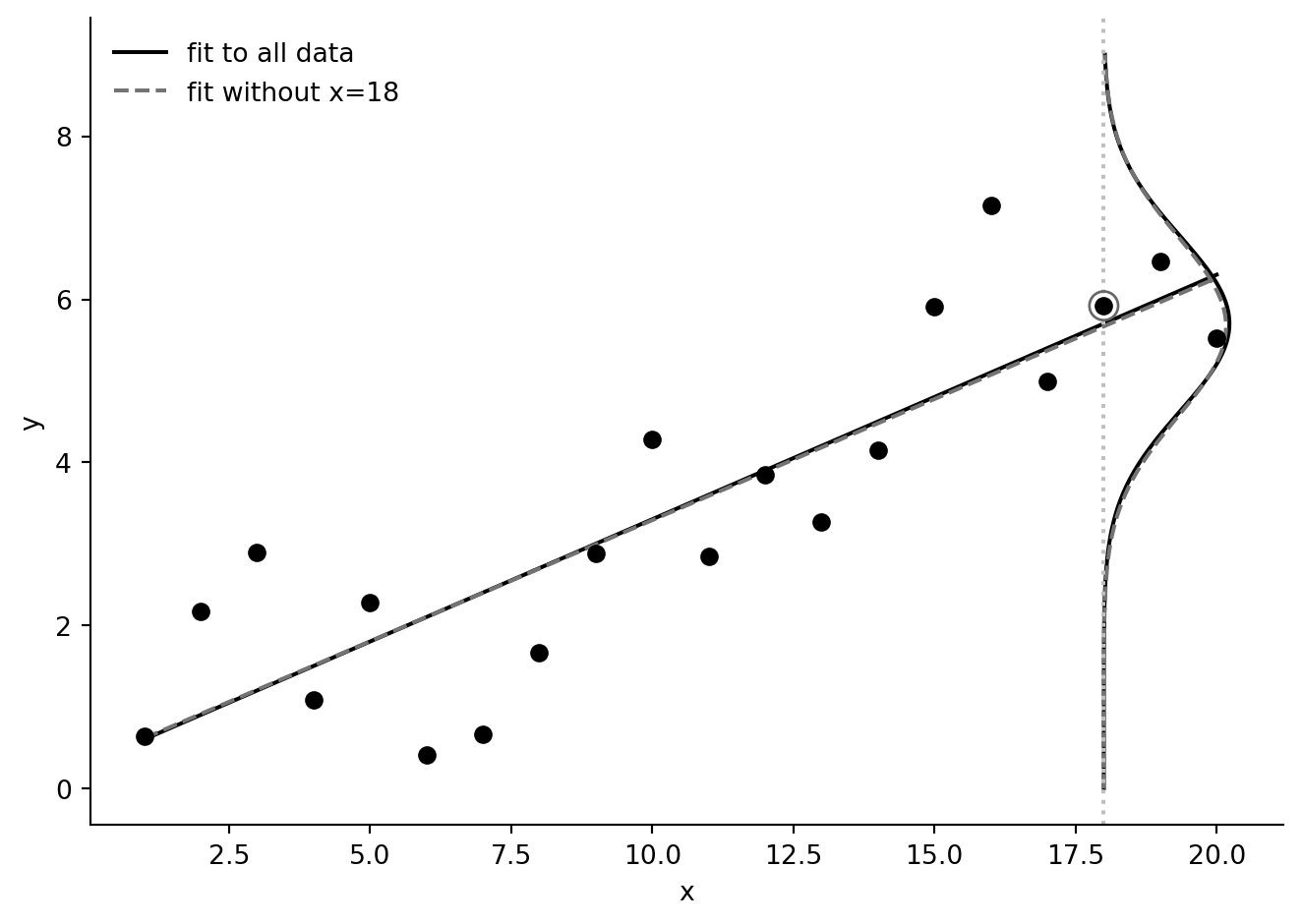
This port keeps the structure of the ROS example: first a tiny simulation showing how leaving out an influential point changes prediction at that point, then the KidIQ comparison where in-sample fit is contrasted with leave-one-out predictive performance. `statsmodels` gives transparent linear-model calculations; ArviZ/CmdStanPy code is included for the Stan-backed PSIS-LOO workflow used by the R `loo` package.
## Setup
```{python}
from pathlib import Path
import sys
import numpy as np
import pandas as pd
import matplotlib.pyplot as plt
import statsmodels.formula.api as smf
from scipy.stats import norm

sys.path.append(str(Path("..").resolve() / "python"))
from data import ros_path

SEED = 1507
rng = np.random.default_rng(SEED)
```
## Simulated data
```{python}
x = np.arange(1, 21)
n = len(x)
a = 0.2
b = 0.3
sigma = 1.0
rng_fake = np.random.default_rng(2141)
y = a + b * x + rng_fake.normal(0, sigma, size=n)
fake = pd.DataFrame({"x": x, "y": y})

fit_all = smf.ols("y ~ x", data=fake).fit()
fit_minus_18 = smf.ols("y ~ x", data=fake.drop(index=17)).fit()
fit_all.params, fit_minus_18.params
```
## Posterior-predictive-style density at the left-out point
For a Gaussian least-squares model, a quick analogue to the posterior predictive distribution uses the fitted mean and residual standard deviation. The R version averages over draws from `stan_glm`; here the deterministic curve is enough to show how the fit changes when observation 18 is omitted.
```{python}
y_grid = np.linspace(0, 9, 200)
mu_all_18 = fit_all.predict(pd.DataFrame({"x": [18]}))[0]
mu_loo_18 = fit_minus_18.predict(pd.DataFrame({"x": [18]}))[0]
sd_all = np.sqrt(fit_all.scale)
sd_loo = np.sqrt(fit_minus_18.scale)
post_curve = pd.DataFrame({
    "y": y_grid,
    "all_data_density": norm.pdf(y_grid, mu_all_18, sd_all),
    "loo_density": norm.pdf(y_grid, mu_loo_18, sd_loo),
})
post_curve.head()
```
```{python}
fig, ax = plt.subplots(figsize=(7, 5))
ax.scatter(fake["x"], fake["y"], color="black", zorder=3)
ax.scatter(fake.loc[17, "x"], fake.loc[17, "y"], facecolors="none", edgecolors="0.4", s=120, zorder=4)
x_grid = np.linspace(fake["x"].min(), fake["x"].max(), 100)
ax.plot(x_grid, fit_all.params["Intercept"] + fit_all.params["x"] * x_grid, color="black", label="fit to all data")
ax.plot(x_grid, fit_minus_18.params["Intercept"] + fit_minus_18.params["x"] * x_grid, color="0.45", ls="--", label="fit without x=18")
# Scale and rotate the predictive density curves, as in the R graphic.
scale = 6.0
ax.plot(18 + scale * post_curve["all_data_density"], post_curve["y"], color="black")
ax.plot(18 + scale * post_curve["loo_density"], post_curve["y"], color="0.45", ls="--")
ax.axvline(18, color="0.75", ls=":")
ax.set(xlabel="x", ylabel="y")
ax.legend(frameon=False)
ax.spines[["top", "right"]].set_visible(False)
fig.tight_layout()
```
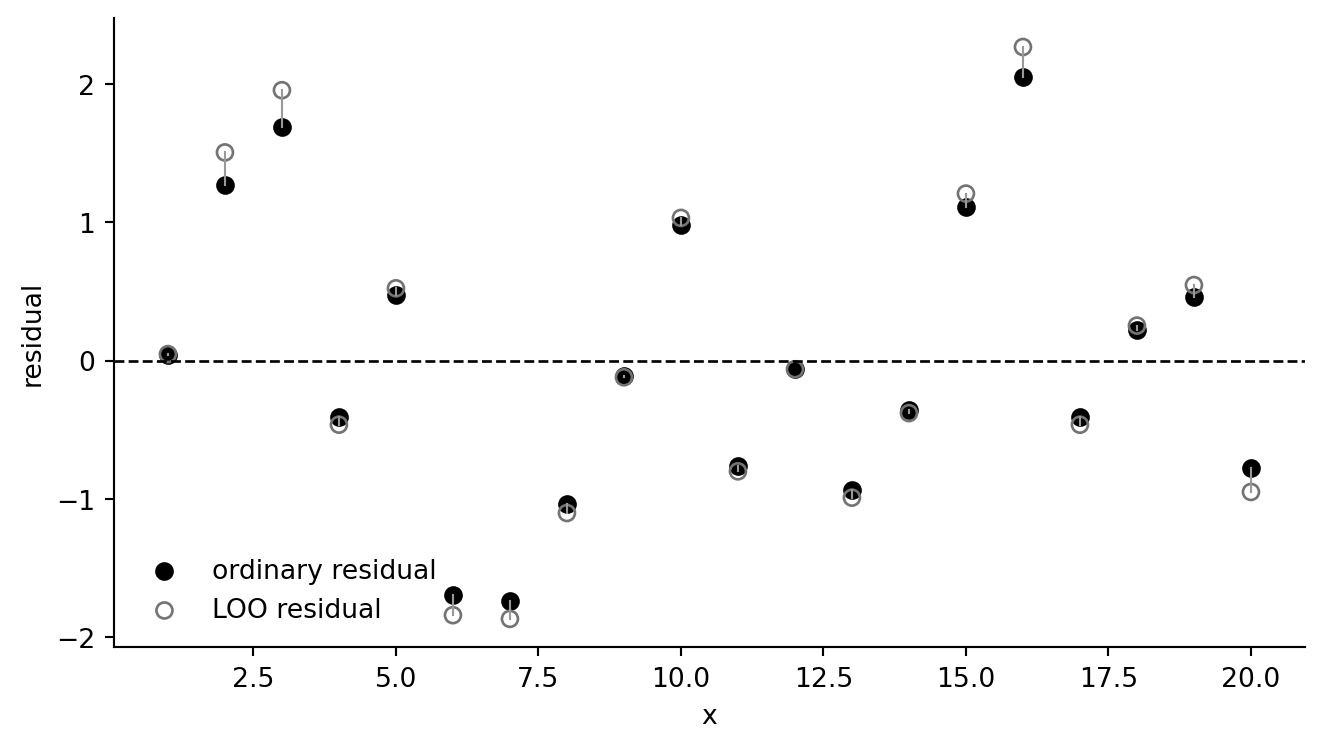
## Ordinary residuals and exact leave-one-out residuals
For linear regression, exact leave-one-out fitted values can be computed from the hat diagonal without refitting the model `n` times:
\[
\hat y_{i,-i} = y_i - \frac{e_i}{1-h_i}.
\]
```{python}
influence = fit_all.get_influence()
fake["residual"] = fit_all.resid
fake["hat"] = influence.hat_matrix_diag
fake["looresidual"] = fake["residual"] / (1 - fake["hat"])
fake["loo_fitted"] = fake["y"] - fake["looresidual"]

round(fake["residual"].std(ddof=1), 2), round(fake["looresidual"].std(ddof=1), 2)
```
```{python}
fig, ax = plt.subplots(figsize=(7, 4))
ax.scatter(fake["x"], fake["residual"], color="black", label="ordinary residual")
ax.scatter(fake["x"], fake["looresidual"], facecolors="none", edgecolors="0.45", label="LOO residual")
for row in fake.itertuples(index=False):
    ax.plot([row.x, row.x], [row.residual, row.looresidual], color="0.6", lw=0.8)
ax.axhline(0, color="black", ls="--", lw=1)
ax.set(xlabel="x", ylabel="residual")
ax.legend(frameon=False)
ax.spines[["top", "right"]].set_visible(False)
fig.tight_layout()
```
```{python}
r2_in_sample = 1 - fake["residual"].var(ddof=1) / fake["y"].var(ddof=1)
r2_loo = 1 - fake["looresidual"].var(ddof=1) / fake["y"].var(ddof=1)
round(r2_in_sample, 2), round(r2_loo, 2)
```
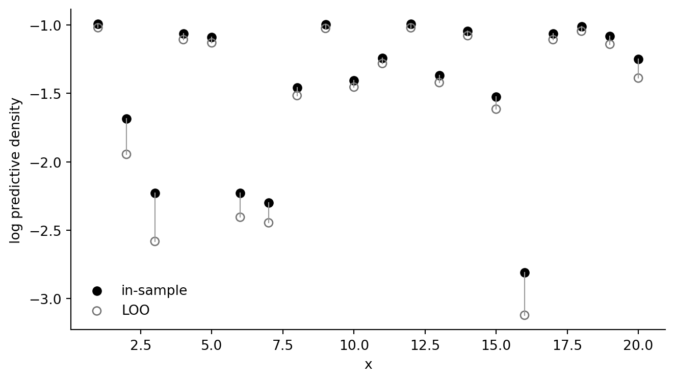
## Log predictive densities
```{python}
fake["lpd_post"] = norm.logpdf(fake["y"], loc=fit_all.fittedvalues, scale=sd_all)
fake["lpd_loo_exact"] = norm.logpdf(fake["y"], loc=fake["loo_fitted"], scale=sd_loo)
fake[["x", "lpd_post", "lpd_loo_exact"]].head()
```
```{python}
fig, ax = plt.subplots(figsize=(7, 4))
ax.scatter(fake["x"], fake["lpd_post"], color="black", label="in-sample")
ax.scatter(fake["x"], fake["lpd_loo_exact"], facecolors="none", edgecolors="0.45", label="LOO")
for row in fake.itertuples(index=False):
    ax.plot([row.x, row.x], [row.lpd_post, row.lpd_loo_exact], color="0.6", lw=0.8)
ax.set(xlabel="x", ylabel="log predictive density")
ax.legend(frameon=False)
ax.spines[["top", "right"]].set_visible(False)
fig.tight_layout()
```
## KidIQ example
```{python}
kidiq = pd.read_csv(ros_path("KidIQ", "data", "kidiq.csv"))
fit_1 = smf.ols("kid_score ~ mom_hs", data=kidiq).fit()
fit_3 = smf.ols("kid_score ~ mom_hs + mom_iq", data=kidiq).fit()

rng = np.random.default_rng(SEED)
kidiqr = kidiq.copy()
for j in range(1, 6):
    kidiqr[f"noise{j}"] = rng.normal(size=len(kidiqr))
noise_terms = " + ".join([f"noise{j}" for j in range(1, 6)])
fit_3n = smf.ols(f"kid_score ~ mom_hs + mom_iq + {noise_terms}", data=kidiqr).fit()
fit_4 = smf.ols("kid_score ~ mom_hs + mom_iq + mom_hs:mom_iq", data=kidiq).fit()
```
```{python}
def loo_residuals_ols(fit):
    h = fit.get_influence().hat_matrix_diag
    return fit.resid / (1 - h)

def loo_r2_ols(fit, y):
    return 1 - np.var(loo_residuals_ols(fit), ddof=1) / np.var(y, ddof=1)

summary = pd.DataFrame({
    "model": ["mom_hs", "mom_hs + mom_iq", "+ five noise predictors", "+ interaction"],
    "in_sample_R2": [fit_1.rsquared, fit_3.rsquared, fit_3n.rsquared, fit_4.rsquared],
    "loo_R2_exact_OLS": [
        loo_r2_ols(fit_1, kidiq["kid_score"]),
        loo_r2_ols(fit_3, kidiq["kid_score"]),
        loo_r2_ols(fit_3n, kidiqr["kid_score"]),
        loo_r2_ols(fit_4, kidiq["kid_score"]),
    ],
})
summary.round(3)
```
The noise predictors can only improve or leave unchanged the in-sample least-squares R2. LOO-R2 penalizes their lack of out-of-sample value through the leverage-adjusted residuals.
## CmdStanPy and ArviZ PSIS-LOO version
The following chunk mirrors the R `stan_glm` + `loo` workflow. It is useful when the model is Bayesian and we want pointwise log likelihoods and Pareto-`k` diagnostics rather than the exact OLS shortcut above.
```{python}
from cmdstanpy import CmdStanModel
import arviz as az
import patsy

stan_dir = Path("_generated_stan")
stan_dir.mkdir(exist_ok=True)
stan_file = stan_dir / "crossvalidation_gaussian_lm.stan"
stan_file.write_text(r'''
data {
  int<lower=1> N;
  int<lower=1> K;
  matrix[N, K] X;
  vector[N] y;
}
parameters {
  vector[K] beta;
  real<lower=0> sigma;
}
model {
  beta ~ normal(0, 20);
  sigma ~ exponential(1.0 / 30);
  y ~ normal(X * beta, sigma);
}
generated quantities {
  vector[N] log_lik;
  for (n in 1:N) log_lik[n] = normal_lpdf(y[n] | dot_product(row(X, n), beta), sigma);
}
''')

# Uncomment to run the Bayesian comparison.
# lm_model = CmdStanModel(stan_file=str(stan_file))
# y3, X3 = patsy.dmatrices("kid_score ~ mom_hs + mom_iq", kidiq, return_type="dataframe")
# fit3_stan = lm_model.sample(
#     data={"N": len(kidiq), "K": X3.shape[1], "X": X3.to_numpy(), "y": np.asarray(y3).ravel()},
#     seed=SEED, chains=4, parallel_chains=4, show_progress=False,
# )
# idata3 = az.from_cmdstanpy(posterior=fit3_stan, log_likelihood="log_lik")
# az.loo(idata3)
```