# Arsenic wells: logistic residuals
Source: `Arsenic/arsenic_logistic_residuals.Rmd`
This ports the ROS binned-residual diagnostics for logistic regression. The fitted models mirror the R formulas through `lapylace` Bernoulli-logit fits, and `matplotlib` recreates the residual checks.
## Setup and data
```{python}
from pathlib import Path
import numpy as np
import pandas as pd
import matplotlib.pyplot as plt
import lapylace as lp
from scipy.special import expit

root = Path("../../ROS-Examples")
wells = pd.read_csv(root / "Arsenic/data/wells.csv")
wells["dist100"] = wells["dist"] / 100
wells["educ4"] = wells["educ"] / 4
wells["c_dist100"] = wells["dist100"] - wells["dist100"].mean()
wells["c_arsenic"] = wells["arsenic"] - wells["arsenic"].mean()
wells["c_educ4"] = wells["educ4"] - wells["educ4"].mean()
wells.head()
```
```{python}
def coef_medians(fit):
    return pd.Series(
        [np.median(fit.alpha_draws()), *np.median(fit.beta_draws(), axis=0)],
        index=["Intercept", *fit.columns],
    )

def posterior_mean_probability(fit, data):
    return fit.posterior_epred(data).mean(axis=0)
```
## Fit the interaction model
```{python}
fit_8 = lp.stan_glm(
    "switch ~ c_dist100 + c_arsenic + c_educ4 + c_dist100:c_educ4 + c_arsenic:c_educ4",
    data=wells,
    family=lp.bernoulli(),
    prior=lp.normal(0, 2.5),
    prior_intercept=lp.normal(0, 5),
    chains=4,
    parallel_chains=4,
    iter_warmup=500,
    iter_sampling=1000,
    seed=15301,
    refresh=100,
)
coef_8 = coef_medians(fit_8)
pred8 = posterior_mean_probability(fit_8, wells)
resid8 = wells["switch"] - pred8
coef_8.round(2)
```
The null classification rule predicts the majority class; the fitted rule classifies by whether the fitted probability is above 0.5.
```{python}
error_rate_null = np.mean(np.round(np.abs(wells["switch"] - pred8.mean())))
error_rate = np.mean(np.round(np.abs(wells["switch"] - pred8)))
round(error_rate_null, 2), round(error_rate, 2)
```
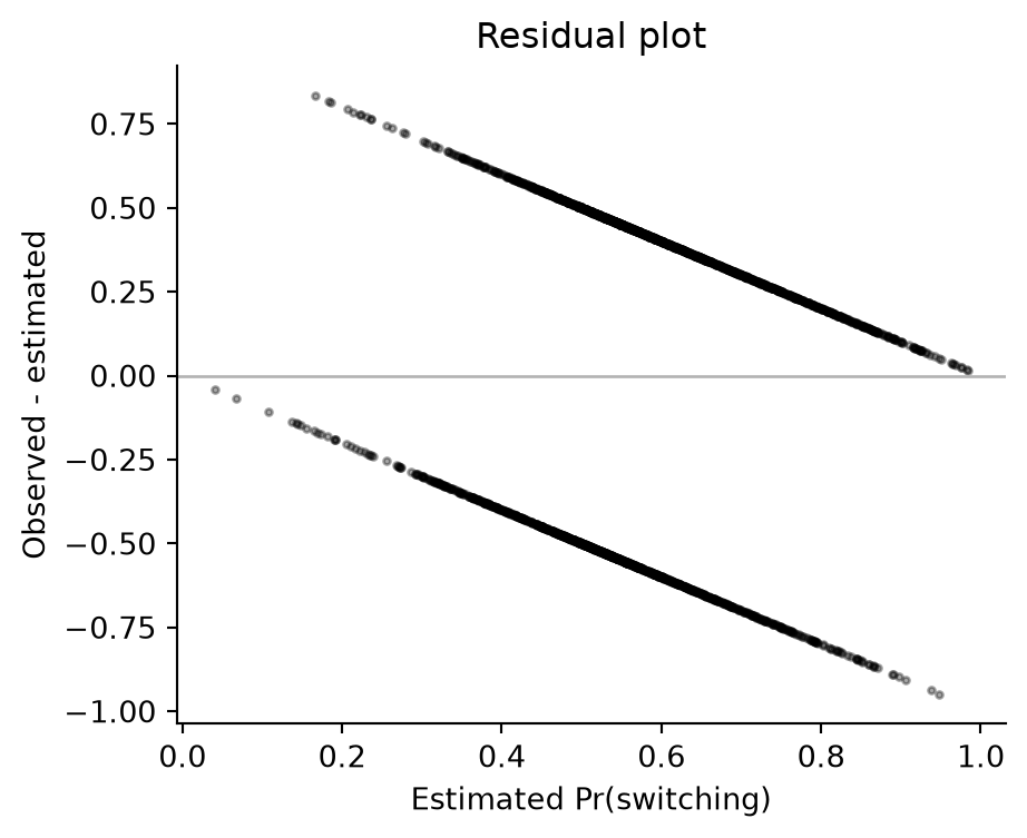
## Raw residual plot
```{python}
fig, ax = plt.subplots(figsize=(5, 4))
ax.axhline(0, color="0.7", lw=1)
ax.scatter(pred8, resid8, s=5, color="black", alpha=0.35)
ax.set(xlabel="Estimated Pr(switching)", ylabel="Observed - estimated", title="Residual plot")
ax.spines[["top", "right"]].set_visible(False)
```
## Binned residuals
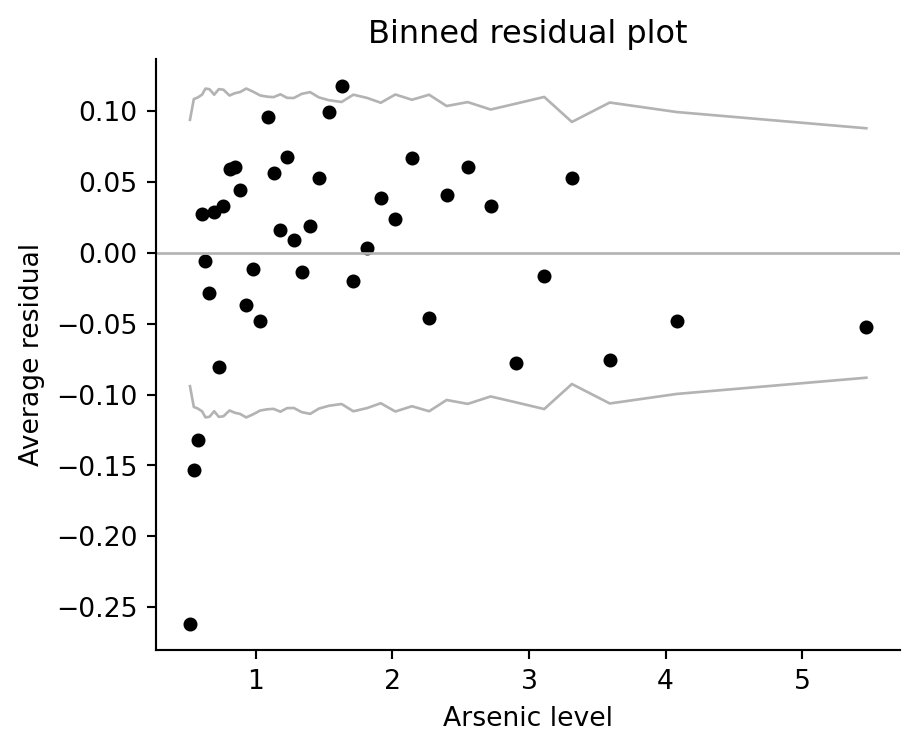
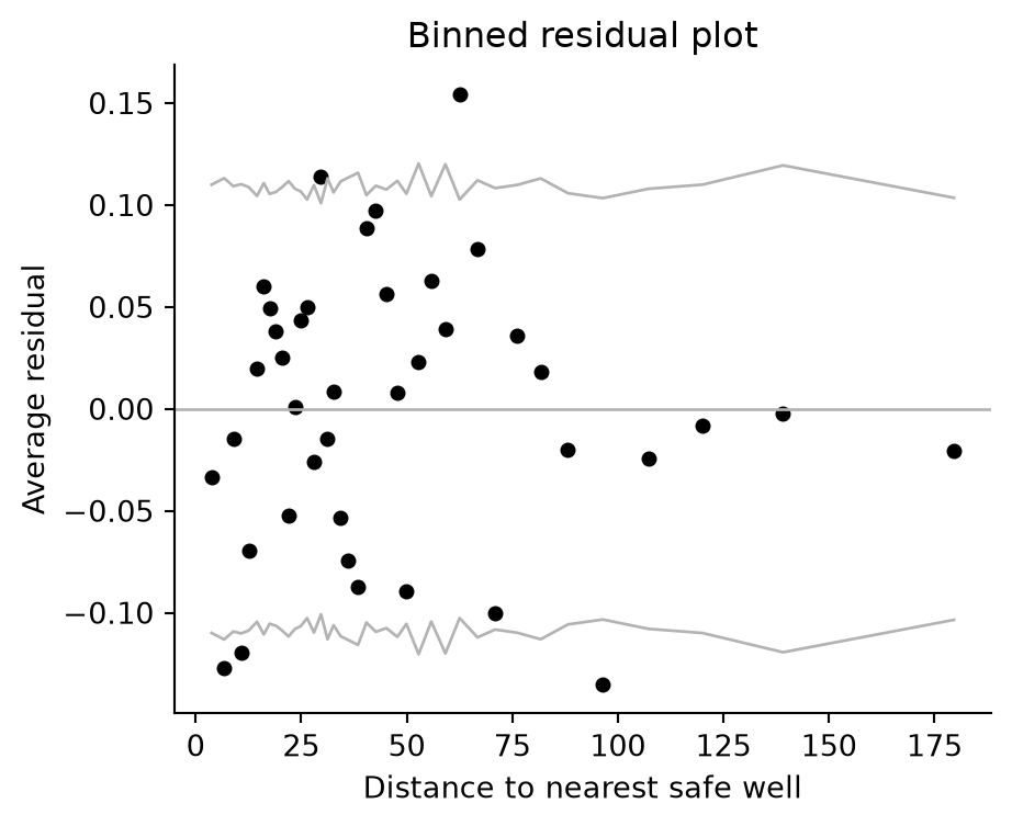
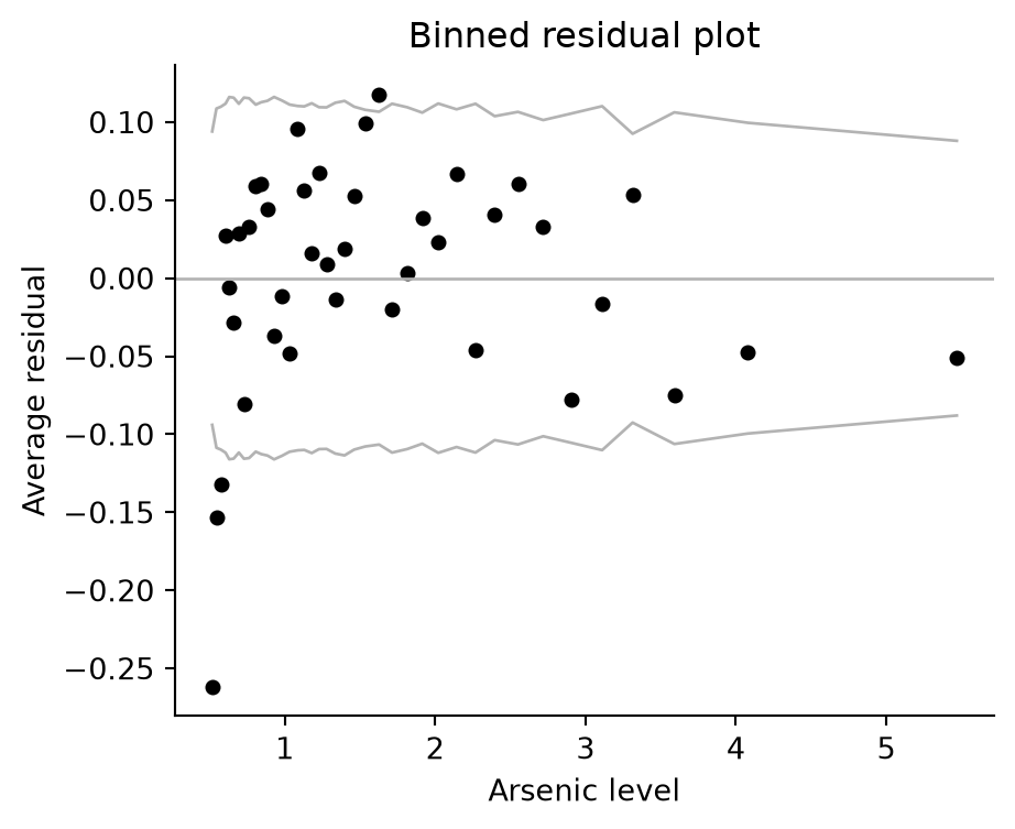
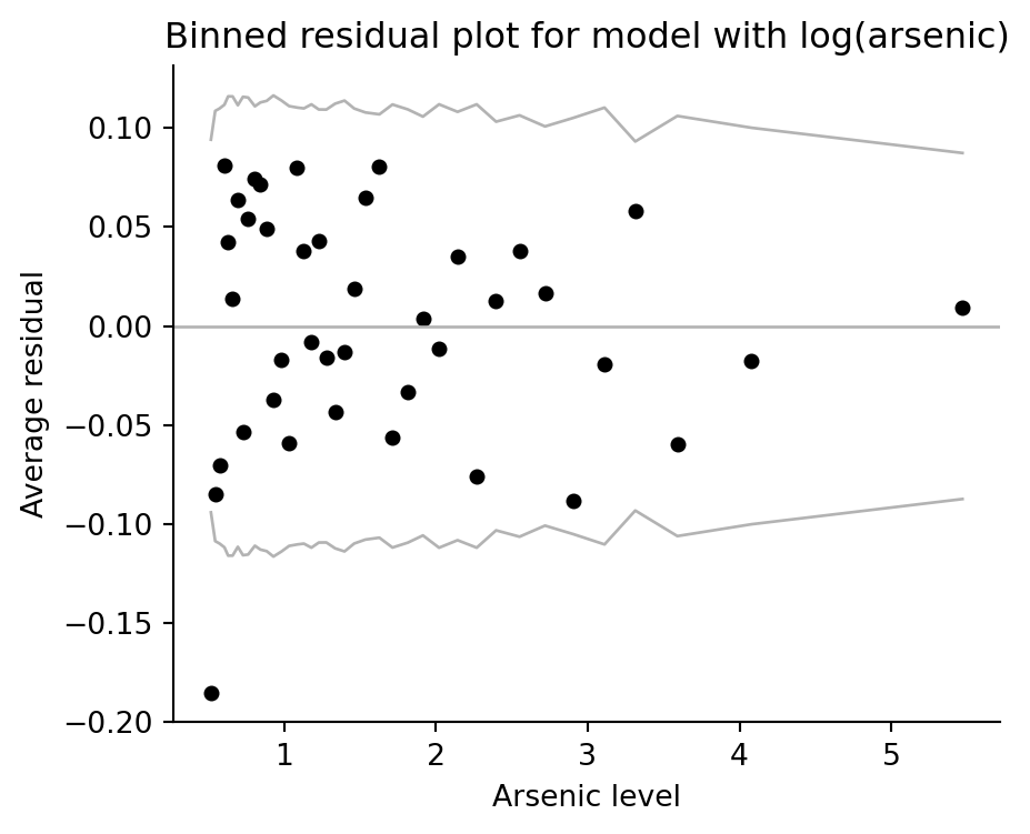
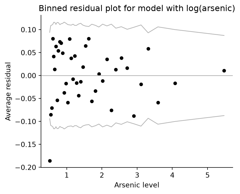
For binary outcomes, raw residuals form two diagonal bands. Binning makes lack of fit easier to see: the average residual in each bin should usually stay inside approximate two-standard-error bands around zero.
```{python}
def binned_resids(x, y, nclass=40):
    x = np.asarray(x)
    y = np.asarray(y)
    order = np.argsort(x)
    groups = np.array_split(order, nclass)
    rows = []
    for idx in groups:
        yy = y[idx]
        xx = x[idx]
        rows.append({
            "xbar": xx.mean(),
            "ybar": yy.mean(),
            "n": len(idx),
            "x_lo": xx.min(),
            "x_hi": xx.max(),
            "two_se": 2 * yy.std(ddof=1) / np.sqrt(len(idx)),
        })
    return pd.DataFrame(rows)

def plot_binned(x, residual, xlabel, title="Binned residual plot", nclass=40):
    br = binned_resids(x, residual, nclass=nclass)
    fig, ax = plt.subplots(figsize=(5, 4))
    ax.axhline(0, color="0.7", lw=1)
    ax.plot(br["xbar"], br["two_se"], color="0.7", lw=1)
    ax.plot(br["xbar"], -br["two_se"], color="0.7", lw=1)
    ax.scatter(br["xbar"], br["ybar"], s=18, color="black")
    ax.set(xlabel=xlabel, ylabel="Average residual", title=title)
    ax.spines[["top", "right"]].set_visible(False)
    return br, ax

br_pred, _ = plot_binned(pred8, resid8, "Estimated Pr(switching)")
br_pred.head()
```
```{python}
br_dist, _ = plot_binned(wells["dist"], resid8, "Distance to nearest safe well")
br_arsenic, _ = plot_binned(wells["arsenic"], resid8, "Arsenic level")
```
## Log-arsenic model
The R example then replaces arsenic with `log(arsenic)` and checks whether the residual pattern against arsenic improves.
```{python}
wells["log_arsenic"] = np.log(wells["arsenic"])
fit_8b = lp.stan_glm(
    "switch ~ dist100 + log_arsenic + educ4 + dist100:educ4 + log_arsenic:educ4",
    data=wells,
    family=lp.bernoulli(),
    prior=lp.normal(0, 2.5),
    prior_intercept=lp.normal(0, 5),
    chains=4,
    parallel_chains=4,
    iter_warmup=500,
    iter_sampling=1000,
    seed=15302,
    refresh=100,
)
coef_8b = coef_medians(fit_8b)
pred8b = posterior_mean_probability(fit_8b, wells)
resid8b = wells["switch"] - pred8b
round(np.mean(np.round(np.abs(wells["switch"] - pred8b))), 2)
```
```{python}
rng = np.random.default_rng(123)
y_jit = wells["switch"] + (1 - 2 * wells["switch"]) * rng.uniform(0, 0.05, len(wells))
xs = np.linspace(0.5, wells["arsenic"].max(), 300)
b = coef_8b
mean_educ4 = wells["educ4"].mean()

fig, ax = plt.subplots(figsize=(5, 4))
ax.scatter(wells["arsenic"], y_jit, s=4, color="black", alpha=0.25)
for dist100, label in [(0, "dist = 0"), (0.5, "dist = 50m")]:
    p = expit(
        b["Intercept"] + b["dist100"] * dist100 + b["log_arsenic"] * np.log(xs)
        + b["educ4"] * mean_educ4 + b["dist100:educ4"] * dist100 * mean_educ4
        + b["log_arsenic:educ4"] * np.log(xs) * mean_educ4
    )
    ax.plot(xs, p, lw=1, label=label)
ax.set(xlabel="Arsenic concentration in well water", ylabel="Pr(switching)")
ax.legend(frameon=False)
ax.spines[["top", "right"]].set_visible(False)
```
```{python}
br_log_arsenic, _ = plot_binned(
    wells["arsenic"], resid8b, "Arsenic level",
    title="Binned residual plot for model with log(arsenic)",
)
```