# Rsquared / rsquared
Source: `Rsquared/rsquared.Rmd`
Gelman, Goodrich, Gabry, and Vehtari define Bayesian R2 draw by draw as
\[
R^2 = \frac{\operatorname{Var}_n(\mu_n)}{\operatorname{Var}_n(\mu_n) + \operatorname{Var}_{\mathrm{res}}},
\]
where `mu` is the model-implied predictive mean. This Python port reproduces the core calculations with `statsmodels` plus normal-approximation posterior draws, and includes a CmdStanPy/ArviZ implementation for exact Bayesian draws when a Stan toolchain is available.
## Setup
```{python}
from pathlib import Path
import sys
import numpy as np
import pandas as pd
import matplotlib.pyplot as plt
import statsmodels.formula.api as smf
import statsmodels.api as sm
from scipy.special import expit

sys.path.append(str(Path("..").resolve() / "python"))
from data import ros_path

SEED = 1800
rng = np.random.default_rng(SEED)
```
## Utility functions
```{python}
def bayes_r2_gaussian(mu_draws, sigma_draws):
    """Bayesian R2 for Gaussian models from posterior draws of mu and sigma."""
    var_mu = np.var(mu_draws, axis=1, ddof=1)
    return var_mu / (var_mu + sigma_draws**2)


def bayes_r2_binary(prob_draws):
    """Tjur/Gelman-style Bayesian R2 for binary models from probability draws."""
    var_mu = np.var(prob_draws, axis=1, ddof=1)
    var_res = np.mean(prob_draws * (1 - prob_draws), axis=1)
    return var_mu / (var_mu + var_res)


def gaussian_draws_from_ols(fit, exog, n_draws=4000, rng=None):
    """Normal approximation to posterior draws for a Gaussian linear model."""
    if rng is None:
        rng = np.random.default_rng()
    beta = rng.multivariate_normal(fit.params.to_numpy(), fit.cov_params().to_numpy(), size=n_draws)
    sigma = np.sqrt(fit.scale) * np.ones(n_draws)
    mu = beta @ np.asarray(exog).T
    return mu, sigma, beta


def binary_draws_from_glm(fit, exog, n_draws=4000, rng=None):
    """Normal approximation to posterior draws for a logistic/probit GLM."""
    if rng is None:
        rng = np.random.default_rng()
    beta = rng.multivariate_normal(np.asarray(fit.params), np.asarray(fit.cov_params()), size=n_draws)
    eta = beta @ np.asarray(exog).T
    if isinstance(fit.family.link, sm.families.links.Probit):
        from scipy.stats import norm
        p = norm.cdf(eta)
    else:
        p = expit(eta)
    return p, beta
```
## Toy data with n=5
```{python}
x = np.arange(1, 6) - 3
y = np.array([1.7, 2.6, 2.5, 4.4, 3.8]) - 3
xy = pd.DataFrame({"x": x, "y": y})

ols = smf.ols("y ~ x", data=xy).fit()
yhat = ols.fittedvalues.to_numpy()
r = y - yhat
rsq_1 = np.var(yhat, ddof=1) / np.var(y, ddof=1)
rsq_2 = np.var(yhat, ddof=1) / (np.var(yhat, ddof=1) + np.var(r, ddof=1))
round(rsq_1, 3), round(rsq_2, 3)
```
The two classical formulas differ in a tiny sample because the fitted values and residuals are not being treated as posterior quantities.
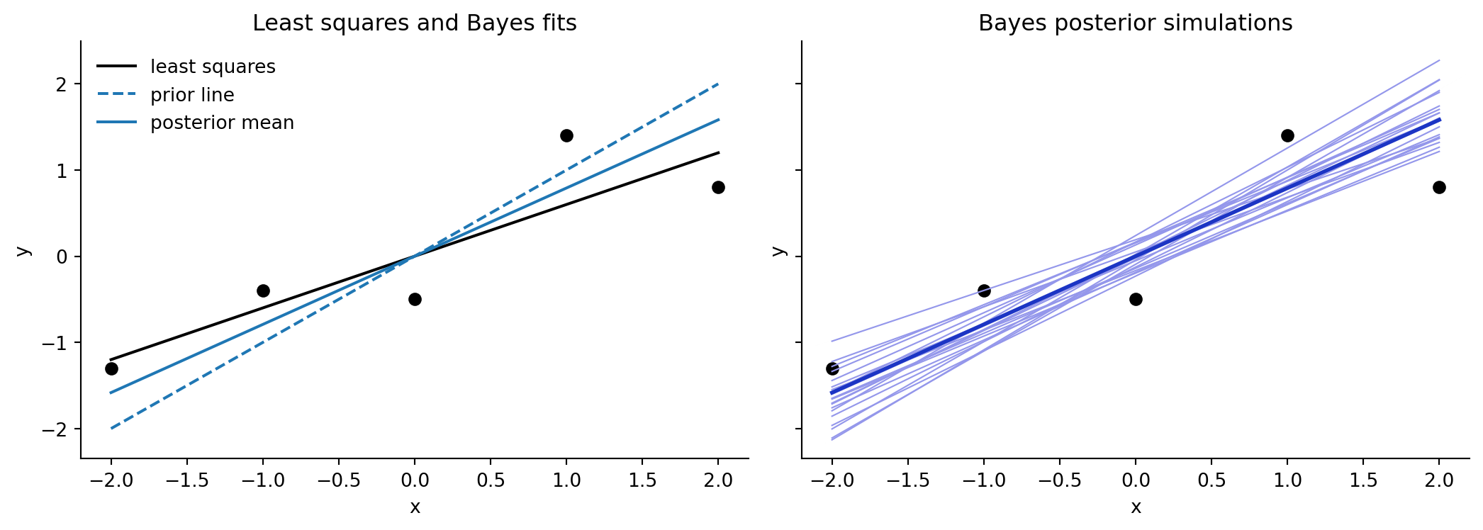
## A prior-pulled Bayesian fit by approximation
The R version fits `stan_glm` with a prior intercept near 0 and slope near 1. The following ridge-posterior approximation encodes the same idea for the five-point example.
```{python}
X = sm.add_constant(x)
prior_mean = np.array([0.0, 1.0])
prior_sd = np.array([0.2, 0.2])
sigma_known = np.sqrt(ols.scale)
prior_precision = np.diag(1 / prior_sd**2)
lik_precision = X.T @ X / sigma_known**2
post_cov = np.linalg.inv(lik_precision + prior_precision)
post_mean = post_cov @ (X.T @ y / sigma_known**2 + prior_precision @ prior_mean)
posterior_beta = rng.multivariate_normal(post_mean, post_cov, size=4000)
mu_draws = posterior_beta @ X.T
sigma_draws = sigma_known * np.ones(len(posterior_beta))
br2_toy = bayes_r2_gaussian(mu_draws, sigma_draws)
round(np.median(br2_toy), 2)
```
```{python}
keep = rng.choice(len(posterior_beta), size=20, replace=False)
fig, axes = plt.subplots(1, 2, figsize=(11, 4), sharex=True, sharey=True)
axes[0].scatter(x, y, color="black")
axes[0].plot(x, ols.params["Intercept"] + ols.params["x"] * x, color="black", label="least squares")
axes[0].plot(x, prior_mean[0] + prior_mean[1] * x, color="tab:blue", ls="--", label="prior line")
axes[0].plot(x, post_mean[0] + post_mean[1] * x, color="tab:blue", label="posterior mean")
axes[0].legend(frameon=False)
axes[0].set_title("Least squares and Bayes fits")

for beta in posterior_beta[keep]:
    axes[1].plot(x, beta[0] + beta[1] * x, color="#9497eb", lw=0.8)
axes[1].plot(x, post_mean[0] + post_mean[1] * x, color="#1c35c4", lw=2)
axes[1].scatter(x, y, color="black")
axes[1].set_title("Bayes posterior simulations")
for ax in axes:
    ax.set(xlabel="x", ylabel="y")
    ax.spines[["top", "right"]].set_visible(False)
fig.tight_layout()
```
```{python}
fig, ax = plt.subplots(figsize=(6, 4))
ax.hist(br2_toy, bins=np.arange(0, 1.02, 0.02), color="0.75", edgecolor="white")
ax.axvline(np.median(br2_toy), color="black")
ax.set(xlabel="Bayesian R2", yticks=[], title="Bayesian R squared posterior and median")
ax.spines[["top", "right", "left"]].set_visible(False)
fig.tight_layout()
```
## Toy logistic regression
```{python}
rng_logit = np.random.default_rng(20)
income = np.arange(1, 21)
rvote = rng_logit.binomial(n=1, p=(income - 0.5) / 20)
toy_logit = pd.DataFrame({"rvote": rvote, "income": income})
fit_logit = smf.glm("rvote ~ income", data=toy_logit, family=sm.families.Binomial()).fit()
prob_draws, _ = binary_draws_from_glm(fit_logit, fit_logit.model.exog, rng=rng)
br2_logit = bayes_r2_binary(prob_draws)
round(np.median(br2_logit), 2)
```
## Mesquite: linear regression
```{python}
mesquite = pd.read_table(ros_path("Mesquite", "data", "mesquite.dat"), sep=r"\s+")
mesquite["canopy_volume"] = mesquite["diam1"] * mesquite["diam2"] * mesquite["canopy_height"]
mesquite["canopy_area"] = mesquite["diam1"] * mesquite["diam2"]
mesquite["canopy_shape"] = mesquite["diam1"] / mesquite["diam2"]
fit_mesquite = smf.ols("np.log(weight) ~ np.log(canopy_volume) + np.log(canopy_shape) + C(group)", data=mesquite).fit()
mu_mesquite, sig_mesquite, _ = gaussian_draws_from_ols(fit_mesquite, fit_mesquite.model.exog, rng=rng)
br2_mesquite = bayes_r2_gaussian(mu_mesquite, sig_mesquite)
round(np.median(br2_mesquite), 2)
```
## Low birth weight: logistic and linear versions
```{python}
lowbwt = pd.read_table(ros_path("LowBwt", "data", "lowbwt.dat"), sep=r"\s+")
fit_low_logit = smf.glm("low ~ age + lwt + C(race) + smoke", data=lowbwt, family=sm.families.Binomial()).fit()
prob_low, _ = binary_draws_from_glm(fit_low_logit, fit_low_logit.model.exog, rng=rng)
br2_low_logit = bayes_r2_binary(prob_low)

fit_low_linear = smf.ols("bwt ~ age + lwt + C(race) + smoke", data=lowbwt).fit()
mu_low, sig_low, _ = gaussian_draws_from_ols(fit_low_linear, fit_low_linear.model.exog, rng=rng)
br2_low_linear = bayes_r2_gaussian(mu_low, sig_low)
round(np.median(br2_low_logit), 2), round(np.median(br2_low_linear), 2)
```
## KidIQ and noise predictors
```{python}
kidiq = pd.read_csv(ros_path("KidIQ", "data", "kidiq.csv"))
fit_kid = smf.ols("kid_score ~ mom_hs + mom_iq", data=kidiq).fit()
mu_kid, sig_kid, _ = gaussian_draws_from_ols(fit_kid, fit_kid.model.exog, rng=rng)
br2_kid = bayes_r2_gaussian(mu_kid, sig_kid)

kidiqr = kidiq.copy()
for j in range(1, 6):
    kidiqr[f"noise{j}"] = rng.normal(size=len(kidiqr))
noise_terms = " + ".join([f"noise{j}" for j in range(1, 6)])
fit_kid_noise = smf.ols(f"kid_score ~ mom_hs + mom_iq + {noise_terms}", data=kidiqr).fit()
mu_kid_noise, sig_kid_noise, _ = gaussian_draws_from_ols(fit_kid_noise, fit_kid_noise.model.exog, rng=rng)
br2_kid_noise = bayes_r2_gaussian(mu_kid_noise, sig_kid_noise)
round(np.median(br2_kid), 2), round(np.median(br2_kid_noise), 2)
```
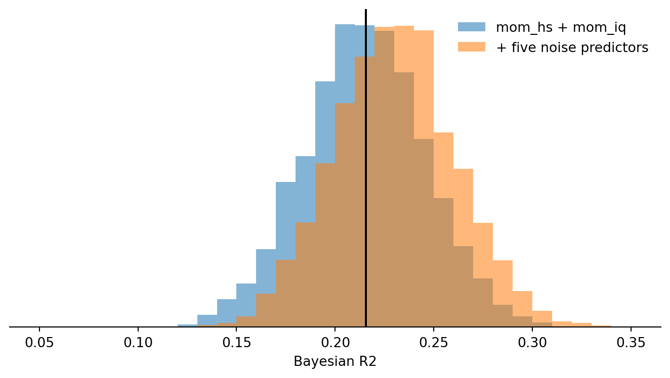
```{python}
fig, ax = plt.subplots(figsize=(7, 4))
ax.hist(br2_kid, bins=np.arange(0.05, 0.36, 0.01), alpha=0.55, label="mom_hs + mom_iq")
ax.hist(br2_kid_noise, bins=np.arange(0.05, 0.36, 0.01), alpha=0.55, label="+ five noise predictors")
ax.axvline(np.median(br2_kid), color="black")
ax.set(xlabel="Bayesian R2", yticks=[])
ax.legend(frameon=False)
ax.spines[["top", "right", "left"]].set_visible(False)
fig.tight_layout()
```
As in the R page, adding pure noise predictors can nudge the in-sample Bayesian R2 upward. The distributional overlap makes clear that this is not a meaningful predictive improvement.
## Earnings: logistic, probit, and positive-earnings linear model
```{python}
earnings = pd.read_csv(ros_path("Earnings", "data", "earnings.csv"))
fit_earn_logit = smf.glm("I(earn > 0) ~ height + male", data=earnings, family=sm.families.Binomial()).fit()
fit_earn_probit = smf.glm(
    "I(earn > 0) ~ height + male",
    data=earnings,
    family=sm.families.Binomial(link=sm.families.links.Probit()),
).fit()
prob_earn_logit, _ = binary_draws_from_glm(fit_earn_logit, fit_earn_logit.model.exog, rng=rng)
prob_earn_probit, _ = binary_draws_from_glm(fit_earn_probit, fit_earn_probit.model.exog, rng=rng)
br2_earn_logit = bayes_r2_binary(prob_earn_logit)
br2_earn_probit = bayes_r2_binary(prob_earn_probit)

positive = earnings[earnings["earn"] > 0].copy()
fit_earn_linear = smf.ols("np.log(earn) ~ height + male", data=positive).fit()
mu_earn, sig_earn, _ = gaussian_draws_from_ols(fit_earn_linear, fit_earn_linear.model.exog, rng=rng)
br2_earn_linear = bayes_r2_gaussian(mu_earn, sig_earn)
round(np.median(br2_earn_logit), 3), round(np.median(br2_earn_probit), 3), round(np.median(br2_earn_linear), 3)
```
The logit and probit versions give nearly the same Bayesian R2 because they imply very similar fitted probabilities for these predictors.
## CmdStanPy implementation for exact posterior draws
For publication-quality Bayesian R2, use posterior draws from Stan rather than the normal approximation above. This Stan program records `mu` and `log_lik`; ArviZ can then summarize both Bayesian R2 and PSIS-LOO from the same fit.
```{python}
from cmdstanpy import CmdStanModel
import arviz as az
import patsy

stan_dir = Path("_generated_stan")
stan_dir.mkdir(exist_ok=True)
stan_file = stan_dir / "rsquared_gaussian_lm.stan"
stan_file.write_text(r'''
data {
  int<lower=1> N;
  int<lower=1> K;
  matrix[N, K] X;
  vector[N] y;
}
parameters {
  vector[K] beta;
  real<lower=0> sigma;
}
model {
  beta ~ normal(0, 20);
  sigma ~ exponential(1.0 / 30);
  y ~ normal(X * beta, sigma);
}
generated quantities {
  vector[N] mu = X * beta;
  vector[N] log_lik;
  for (n in 1:N) log_lik[n] = normal_lpdf(y[n] | mu[n], sigma);
}
''')

# Uncomment to run the KidIQ Bayesian R2 with Stan draws.
# model = CmdStanModel(stan_file=str(stan_file))
# y_stan, X_stan = patsy.dmatrices("kid_score ~ mom_hs + mom_iq", kidiq, return_type="dataframe")
# fit_stan = model.sample(
#     data={"N": len(kidiq), "K": X_stan.shape[1], "X": X_stan.to_numpy(), "y": np.asarray(y_stan).ravel()},
#     seed=SEED, chains=4, parallel_chains=4, show_progress=False,
# )
# draws = fit_stan.draws_pd()
# mu_cols = [f"mu[{i}]" for i in range(1, len(kidiq) + 1)]
# br2_stan = bayes_r2_gaussian(draws[mu_cols].to_numpy(), draws["sigma"].to_numpy())
# idata = az.from_cmdstanpy(posterior=fit_stan, log_likelihood="log_lik")
# np.median(br2_stan), az.loo(idata)
```