Residuals / residuals

Source: Residuals/residuals.Rmd

The original page uses stan_glm, but the displayed ideas are ordinary fitted values and residuals. Here we use statsmodels OLS to reproduce the same simulated examples: first a treatment indicator plus one pre-treatment predictor, then a higher-dimensional predictor matrix where fitted values are the natural one-dimensional summary.

Setup

import numpy as np
import pandas as pd
import matplotlib.pyplot as plt
import statsmodels.formula.api as smf

rng = np.random.default_rng(1507)

One predictor and a treatment indicator

N = 100
x = rng.uniform(0, 1, size=N)
z = rng.integers(0, 2, size=N)
a = 1.0
b = 2.0
theta = 5.0
sigma = 2.0
y = a + b * x + theta * z + rng.normal(0, sigma, size=N)
fake = pd.DataFrame({"x": x, "z": z, "y": y})

fit = smf.ols("y ~ x + z", data=fake).fit()
fit.params

Intercept    0.626230
x            2.497487
z            4.740278
dtype: float64

fig, axes = plt.subplots(1, 2, figsize=(10, 4), sharex=True, sharey=True)
for level, ax in enumerate(axes):
    subset = fake[fake["z"] == level]
    ax.scatter(subset["x"], subset["y"], color="black", marker="o" if level == 0 else "^", s=30)
    x_grid = np.linspace(fake["x"].min(), fake["x"].max(), 100)
    y_grid = fit.params["Intercept"] + fit.params["x"] * x_grid + fit.params["z"] * level
    ax.plot(x_grid, y_grid, color="black")
    ax.set_title(f"z = {level}")
    ax.set_xlabel("Pre-treatment predictor, x")
    ax.spines[["top", "right"]].set_visible(False)
axes[0].set_ylabel("Outcome, y")
fig.tight_layout()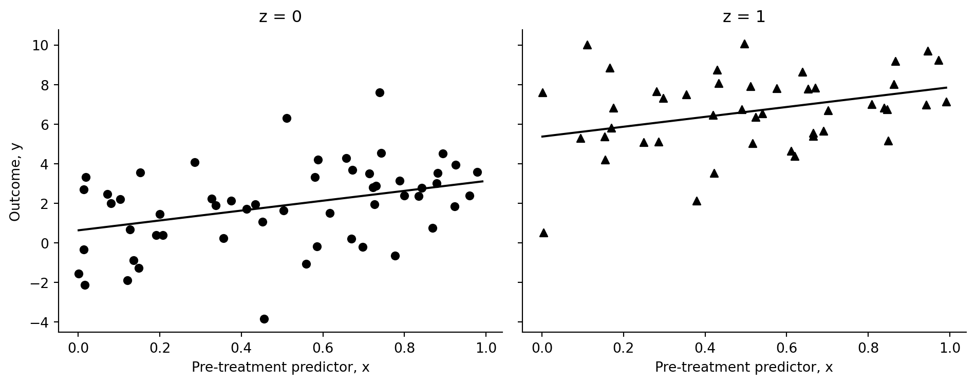

Conditioning on z, the fitted regression line shifts vertically by the estimated treatment coefficient while keeping a common slope for x.

Many pre-treatment predictors

N = 100
K = 10
X = rng.uniform(0, 1, size=(N, K))
z = rng.integers(0, 2, size=N)
a = 1.0
b = np.arange(1, K + 1)
theta = 10.0
sigma = 5.0
y = a + X @ b + theta * z + rng.normal(0, sigma, size=N)

fake_many = pd.DataFrame(X, columns=[f"x{k}" for k in range(1, K + 1)])
fake_many["z"] = z
fake_many["y"] = y
formula = "y ~ " + " + ".join([f"x{k}" for k in range(1, K + 1)]) + " + z"
fit_many = smf.ols(formula, data=fake_many).fit()
fake_many["y_hat"] = fit_many.fittedvalues
fake_many["residual"] = fit_many.resid
fit_many.rsquared

np.float64(0.698002161538674)

Outcome against the linear predictor

lims = [min(fake_many["y"].min(), fake_many["y_hat"].min()), max(fake_many["y"].max(), fake_many["y_hat"].max())]
fig, axes = plt.subplots(1, 2, figsize=(10, 4), sharex=True, sharey=True)
for level, ax in enumerate(axes):
    subset = fake_many[fake_many["z"] == level]
    ax.scatter(subset["y_hat"], subset["y"], color="black", marker="o" if level == 0 else "^", s=30)
    ax.plot(lims, lims, color="black", lw=1)
    ax.set_title(f"z = {level}")
    ax.set_xlabel(r"Linear predictor, $\hat y$")
    ax.spines[["top", "right"]].set_visible(False)
axes[0].set_ylabel("Outcome, y")
fig.tight_layout()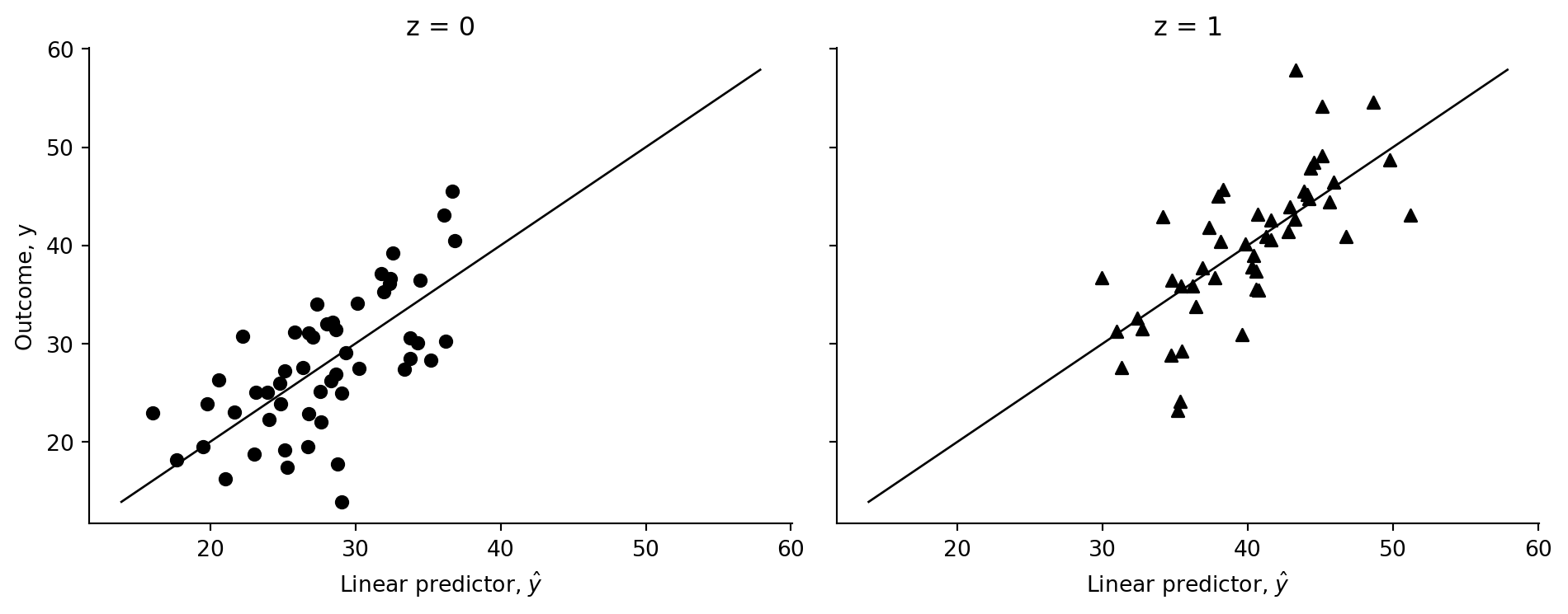

Residuals against the linear predictor

fig, axes = plt.subplots(1, 2, figsize=(10, 4), sharex=True, sharey=True)
for level, ax in enumerate(axes):
    subset = fake_many[fake_many["z"] == level]
    ax.scatter(subset["y_hat"], subset["residual"], color="black", marker="o" if level == 0 else "^", s=30)
    ax.axhline(0, color="black", lw=1)
    ax.set_title(f"z = {level}")
    ax.set_xlabel(r"Linear predictor, $\hat y$")
    ax.spines[["top", "right"]].set_visible(False)
axes[0].set_ylabel("Residual, r")
fig.tight_layout()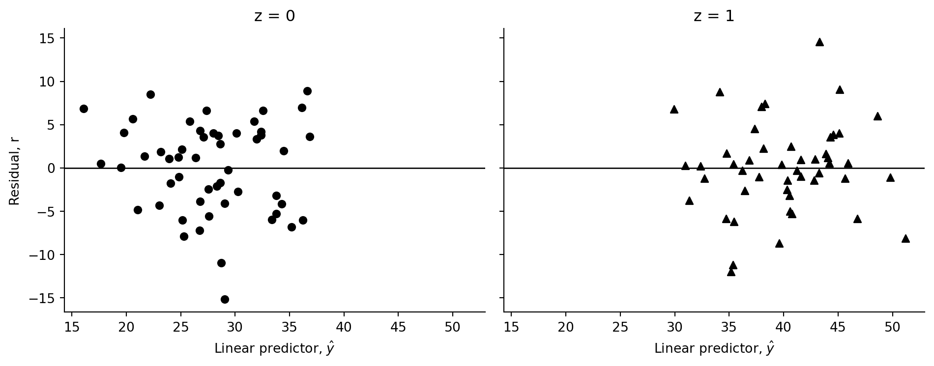

The residual plot removes the fitted mean structure. The remaining vertical scatter is what the Gaussian error term represents in this simulated example.