from pathlib import Path
import numpy as np
import pandas as pd
import matplotlib.pyplot as plt
import lapylace as lp

root = Path("../../ROS-Examples")

def coef_medians(fit):
    return pd.Series(
        [np.median(fit.alpha_draws()), *np.median(fit.beta_draws(), axis=0)],
        index=["Intercept", *fit.columns],
    )

def fit_glm(formula, data, family=None, seed=1, prior_scale=2.5, intercept_scale=5, aux_scale=10, **kwargs):
    return lp.stan_glm(
        formula,
        data=data,
        family=family or lp.gaussian(),
        prior=lp.normal(0, prior_scale),
        prior_intercept=lp.normal(0, intercept_scale),
        prior_aux=lp.exponential(aux_scale),
        chains=2,
        parallel_chains=2,
        iter_warmup=300,
        iter_sampling=500,
        seed=seed,
        refresh=100,
        **kwargs,
)Earnings: regression examples
Source: Earnings/earnings_regression.Rmd
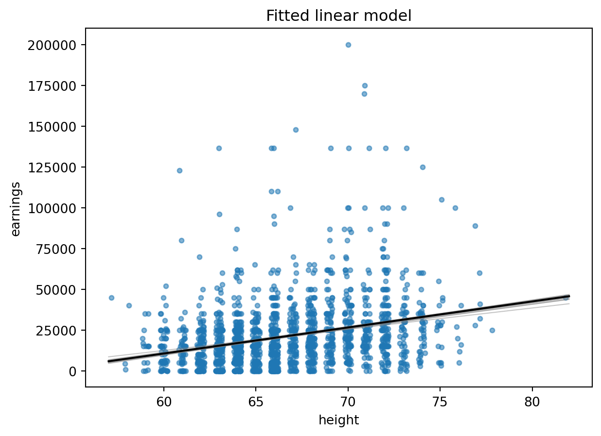
The page fits the earnings regressions with Bayesian Gaussian models in lapylace, using the same formulas as the original stan_glm examples.
Setup
earnings = pd.read_csv(root / "Earnings/data/earnings.csv")
earnings = earnings.dropna(subset=["earn", "earnk", "height", "male"])
earnings["log_earn"] = np.log(earnings["earn"].clip(lower=1))
earnings.head()| height | weight | male | earn | earnk | ethnicity | education | mother_education | father_education | walk | exercise | smokenow | tense | angry | age | log_earn | |
|---|---|---|---|---|---|---|---|---|---|---|---|---|---|---|---|---|
| 0 | 74 | 210.0 | 1 | 50000.0 | 50.0 | White | 16.0 | 16.0 | 16.0 | 3 | 3 | 2.0 | 0.0 | 0.0 | 45 | 10.819778 |
| 1 | 66 | 125.0 | 0 | 60000.0 | 60.0 | White | 16.0 | 16.0 | 16.0 | 6 | 5 | 1.0 | 0.0 | 0.0 | 58 | 11.002100 |
| 2 | 64 | 126.0 | 0 | 30000.0 | 30.0 | White | 16.0 | 16.0 | 16.0 | 8 | 1 | 2.0 | 1.0 | 1.0 | 29 | 10.308953 |
| 3 | 65 | 200.0 | 0 | 25000.0 | 25.0 | White | 17.0 | 17.0 | NaN | 8 | 1 | 2.0 | 0.0 | 0.0 | 57 | 10.126631 |
| 4 | 63 | 110.0 | 0 | 50000.0 | 50.0 | Other | 16.0 | 16.0 | 16.0 | 5 | 6 | 2.0 | 0.0 | 0.0 | 91 | 10.819778 |
models = {
    "earnk ~ height": fit_glm("earnk ~ height", earnings, seed=17501, prior_scale=10, intercept_scale=100, aux_scale=50),
    "earnk ~ height + male": fit_glm("earnk ~ height + male", earnings, seed=17502, prior_scale=10, intercept_scale=100, aux_scale=50),
    "log_earn ~ height + male": fit_glm("log_earn ~ height + male", earnings, seed=17503, prior_scale=2.5, intercept_scale=10, aux_scale=5),
}
pd.concat({name: coef_medians(fit) for name, fit in models.items()}, axis=1).round(3) | earnk ~ height | earnk ~ height + male | log_earn ~ height + male | |
|---|---|---|---|
| Intercept | -84.076 | -27.487 | 2.972 |
| height | 1.581 | 0.671 | 0.079 |
| male | NaN | 10.434 | 1.271 |
grid = pd.DataFrame({"height": np.linspace(earnings.height.min(), earnings.height.max(), 120), "male": 1})
pred = models["earnk ~ height + male"].posterior_epred(grid)
fig, ax = plt.subplots()
ax.scatter(earnings.height, earnings.earnk, alpha=.2, s=10)
ax.plot(grid.height, pred.mean(axis=0), color="black")
ax.set_xlabel("Height")
ax.set_ylabel("Earnings, thousands")
Text(0, 0.5, 'Earnings, thousands')