# Golf putting accuracy
Source: `Golf/golf.Rmd`
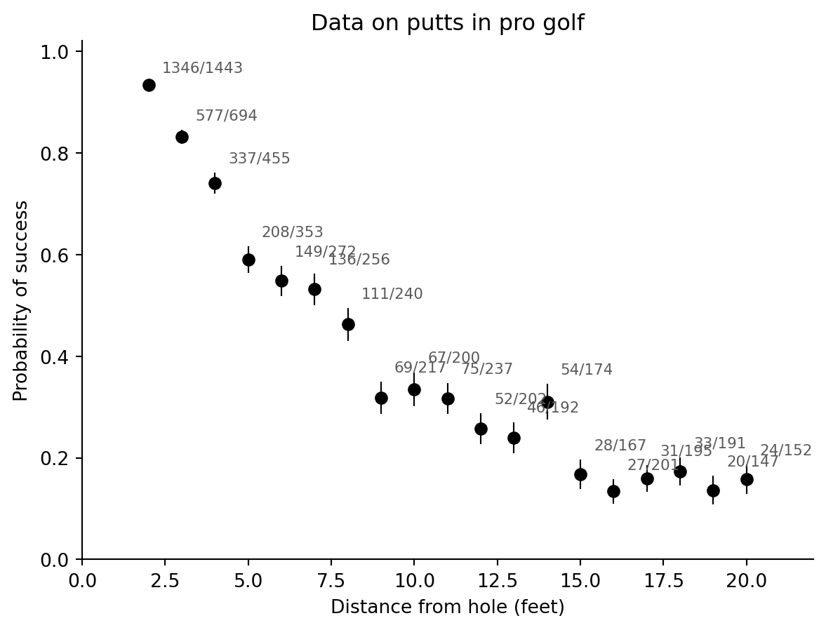
This page ports the ROS golf-putting example to Python. The data are binomial counts of successful putts at different distances. We fit a Bayesian logistic regression and the geometry-based model from the book, where putt success is driven by angular error.
```{python}
from pathlib import Path
import numpy as np
import pandas as pd
import matplotlib.pyplot as plt
from scipy.special import expit, logit
from scipy.stats import norm, binom, halfnorm
from python.bayes_glm import bayes_logit

root = Path("../../ROS-Examples")
golf_dir = root / "Golf"
golf = pd.read_csv(golf_dir / "data/golf.txt", sep=r"\s+", skiprows=2)
golf["p_hat"] = golf["y"] / golf["n"]
golf["se"] = np.sqrt(golf["p_hat"] * (1 - golf["p_hat"]) / golf["n"])
r = (1.68 / 2) / 12
R = (4.25 / 2) / 12
golf.head()
```
## Plot the data
```{python}
fig, ax = plt.subplots(figsize=(7, 5))
ax.errorbar(golf.x, golf.p_hat, yerr=golf.se, fmt="o", color="black", lw=0.8)
for _, row in golf.iterrows():
    ax.text(row.x + 0.4, row.p_hat + row.se + 0.02, f"{int(row.y)}/{int(row.n)}", fontsize=8, color="0.35")
ax.set(xlim=(0, 1.1 * golf.x.max()), ylim=(0, 1.02), xlabel="Distance from hole (feet)", ylabel="Probability of success", title="Data on putts in pro golf")
ax.spines[["top", "right"]].set_visible(False)
```
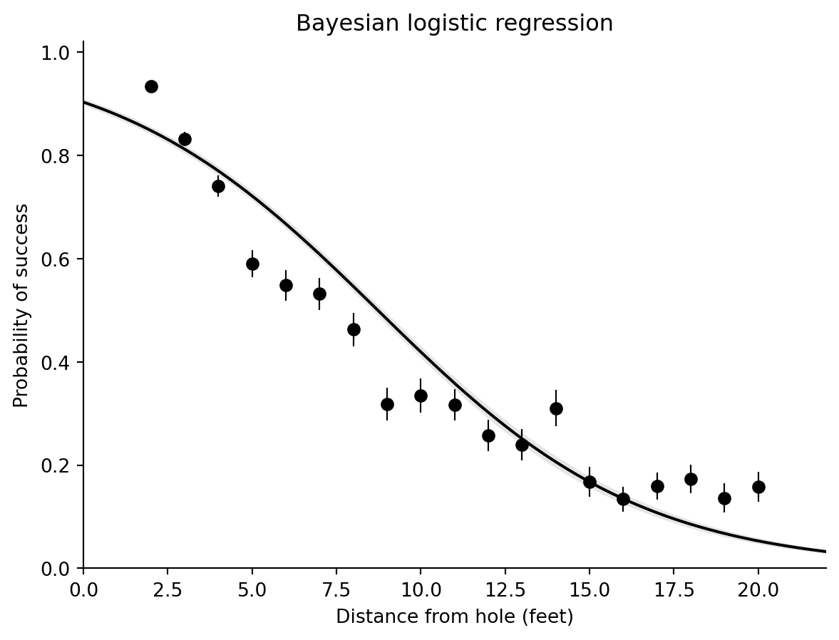
## Bayesian logistic regression
The R page uses `rstanarm::stan_glm(cbind(y, n-y) ~ x, family=binomial)`. For a fast executed port we expand the grouped binomial counts to Bernoulli rows and fit a Normal-prior Bayesian logistic regression via the shared `bayes_logit` helper.
```{python}
expanded = pd.DataFrame({
    "x": np.repeat(golf.x.to_numpy(), golf.n.astype(int).to_numpy()),
    "made": np.concatenate([np.r_[np.ones(int(y)), np.zeros(int(n-y))] for y, n in zip(golf.y, golf.n)]).astype(int),
})
fit_logit = bayes_logit("made ~ x", expanded, draws=3000, prior_scale=2.5, seed=1507)
fit_logit.summary().round(3)
```
```{python}
x_grid = np.linspace(0, 1.1 * golf.x.max(), 300)
p_draws = fit_logit.epred(pd.DataFrame({"x": x_grid}))
p_logit = np.median(p_draws, axis=0)
p_band = np.quantile(p_draws, [0.1, 0.9], axis=0)

fig, ax = plt.subplots(figsize=(7, 5))
ax.errorbar(golf.x, golf.p_hat, yerr=golf.se, fmt="o", color="black", lw=0.8)
ax.plot(x_grid, p_logit, color="black")
ax.fill_between(x_grid, p_band[0], p_band[1], color="gray", alpha=.2, linewidth=0)
ax.set(xlim=(0, 1.1 * golf.x.max()), ylim=(0, 1.02), xlabel="Distance from hole (feet)", ylabel="Probability of success", title="Bayesian logistic regression")
ax.spines[["top", "right"]].set_visible(False)
```
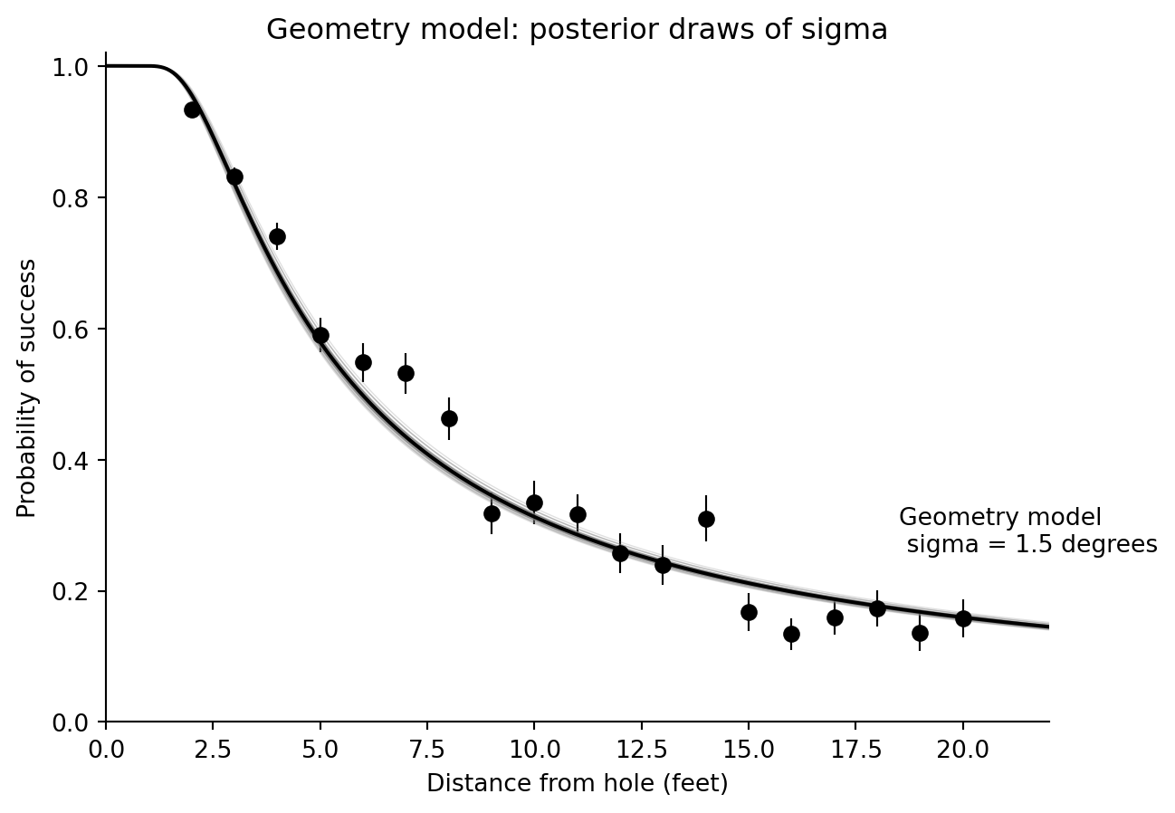
## Geometry-based nonlinear model
The custom model uses the angle subtended by the effective target, `asin((R-r)/x)`, and a single angular-error parameter `sigma`:
$$
p(x;\sigma) = 2\Phi\left(\frac{\sin^{-1}((R-r)/x)}{\sigma}\right)-1.
$$
We compute the one-dimensional posterior on a grid with a weak half-normal prior for `sigma`.
```{python}
def p_geometry(x, sigma):
    x = np.asarray(x, dtype=float)
    p = np.ones_like(x, dtype=float)
    ok = x > (R - r)
    p[ok] = 2 * norm.cdf(np.arcsin((R - r) / x[ok]) / sigma) - 1
    return np.clip(p, 1e-9, 1-1e-9)

sigma_grid = np.linspace(0.005, 0.30, 3000)
log_prior = halfnorm(scale=0.10).logpdf(sigma_grid)
log_lik = np.array([
    np.sum(binom.logpmf(golf.y, golf.n, p_geometry(golf.x, sig)))
    for sig in sigma_grid
])
log_post = log_prior + log_lik
post = np.exp(log_post - log_post.max())
post = post / np.trapezoid(post, sigma_grid)
cdf = np.cumsum(post); cdf = cdf / cdf[-1]
rng = np.random.default_rng(1507)
sigma_draws = np.interp(rng.uniform(size=3000), cdf, sigma_grid)
sigma_hat = np.median(sigma_draws)
sigma_hat, sigma_hat * 180 / np.pi
```
```{python}
x_geom = np.linspace(R - r, 1.1 * golf.x.max(), 300)
fig, ax = plt.subplots(figsize=(7, 5))
ax.errorbar(golf.x, golf.p_hat, yerr=golf.se, fmt="o", color="black", lw=0.8)
for sigma in sigma_draws[:60]:
    ax.plot(np.r_[0, R-r, x_geom], np.r_[1, 1, p_geometry(x_geom, sigma)], color="0.5", lw=0.5, alpha=0.25)
ax.plot(np.r_[0, R-r, x_geom], np.r_[1, 1, p_geometry(x_geom, sigma_hat)], color="black", lw=1.5)
ax.text(18.5, 0.26, f"Geometry model\n sigma = {sigma_hat * 180 / np.pi:.1f} degrees")
ax.set(xlim=(0, 1.1 * golf.x.max()), ylim=(0, 1.02), xlabel="Distance from hole (feet)", ylabel="Probability of success", title="Geometry model: posterior draws of sigma")
ax.spines[["top", "right"]].set_visible(False)
```
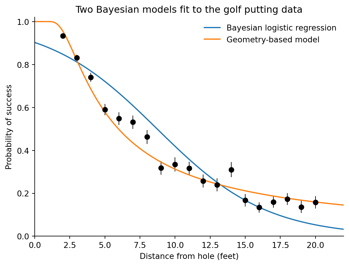
## Model comparison plot
```{python}
fig, ax = plt.subplots(figsize=(7, 5))
ax.errorbar(golf.x, golf.p_hat, yerr=golf.se, fmt="o", color="black", lw=0.8)
ax.plot(x_grid, p_logit, label="Bayesian logistic regression")
ax.plot(np.r_[0, R-r, x_geom], np.r_[1, 1, p_geometry(x_geom, sigma_hat)], label="Geometry-based model")
ax.set(xlim=(0, 1.1 * golf.x.max()), ylim=(0, 1.02), xlabel="Distance from hole (feet)", ylabel="Probability of success", title="Two Bayesian models fit to the golf putting data")
ax.legend(frameon=False)
ax.spines[["top", "right"]].set_visible(False)
```
## Log-density sketch
The geometry model is also a natural example for custom samplers: the log density over `log_sigma` is just the binomial likelihood plus the prior and Jacobian.
```{python}
def golf_geometry_logdensity(log_sigma):
    sigma = np.exp(log_sigma)
    p = p_geometry(golf.x, sigma)
    return np.sum(binom.logpmf(golf.y, golf.n, p)) + halfnorm(scale=0.10).logpdf(sigma) + log_sigma

golf_geometry_logdensity(np.log(sigma_hat))
```