# Pew survey recodes and weighted income profiles
Source: `Pew/pew.Rmd`
The source page is a collection of data-cleaning and visualization steps for raw Pew 2008 election survey data. This port focuses on the core workflow: read the Stata file, recreate the vote-intention and weighting variables, recode income/party/ideology/religious-attendance scales, and reproduce the weighted income profiles.
## Setup and data
```{python}
from pathlib import Path
import numpy as np
import pandas as pd
import matplotlib.pyplot as plt

root = Path("/Users/alal/tmp/ros-python-book/ROS-Examples")
pew_pre = pd.read_stata(root / "Pew/data/pew_research_center_june_elect_wknd_data.dta", convert_categoricals=True)
n = len(pew_pre)
pew_pre[["date", "heat2", "heat4", "regicert", "state", "weight", "income", "party", "partyln", "ideo"]].head()
```
```{python}
which_question = np.where(pew_pre["heat2"].notna(), 2, np.where(pew_pre["heat4"].notna(), 4, 0))
pd.crosstab(pew_pre["date"], which_question).head()
```
## Vote intention and registration
The R source creates `rvote = 1` for Republican/lean-Republican vote intention and `rvote = 0` for Democratic/lean-Democratic vote intention, using whichever of `heat2` or `heat4` was asked.
```{python}
def norm_text(s):
    return s.astype("string").str.lower().str.strip()

heat2 = norm_text(pew_pre["heat2"])
heat4 = norm_text(pew_pre["heat4"])
rvote = pd.Series(np.nan, index=pew_pre.index, dtype="float")
rvote = rvote.mask((which_question == 2) & heat2.eq("rep/lean rep"), 1)
rvote = rvote.mask((which_question == 2) & heat2.eq("dem/lean dem"), 0)
rvote = rvote.mask((which_question == 4) & heat4.eq("rep/lean rep"), 1)
rvote = rvote.mask((which_question == 4) & heat4.eq("dem/lean dem"), 0)

registered = norm_text(pew_pre["regicert"]).eq("absolutely certain").fillna(False).astype(int)
pd.Series({"observations": n, "major-party vote intentions": rvote.notna().sum(), "certain registered": registered.sum()})
```
## Dates, poll IDs, and weights
The poll identifier follows the nested date cutoffs in the R code. Weights are normalized within each poll wave; `voter_weight` is only defined for registered respondents with a major-party vote intention.
```{python}
date = pew_pre["date"].astype(int)
month = date // 10000
day = date // 100 - 100 * month
poll_id = np.select(
    [
        month == 6,
        (month == 7) & (day < 28),
        ((month == 7) & (day >= 28)) | (month == 8),
        (month == 9) & (day < 16),
        (month == 9) & (day >= 16),
        (month == 10) & (day < 14),
        (month == 10) & (day >= 14) & (day < 20),
        (month == 10) & (day >= 20) & (day < 27),
    ],
    [1, 2, 3, 4, 5, 6, 7, 8],
    default=9,
)

pop_weight0 = pew_pre["weight"].astype(float)
voter_weight0 = pop_weight0.where(rvote.notna() & registered.eq(1))

pop_weight = pop_weight0 / pop_weight0.groupby(poll_id).transform("mean")
voter_weight = voter_weight0 / voter_weight0.groupby(poll_id).transform("mean")

pd.DataFrame({"poll_id": poll_id, "pop_weight": pop_weight, "voter_weight": voter_weight}).groupby("poll_id").mean().round(3)
```
## Income, party identification, and ideology recodes
The labels in the Stata file are already readable strings, so the Python recodes map those labels directly rather than relying on R factor codes.
```{python}
income_order = [
    "less than $10,000", "$10,000-$19,999", "$20,000-$29,999", "$30,000-$39,999",
    "$40,000-$49,999", "$50,000-$74,999", "$75,000-$99,999", "$100,000-$149,999", "$150,000 or more",
]
income_map = {label: i + 1 for i, label in enumerate(income_order)}
inc = norm_text(pew_pre["income"]).map({k.lower(): v for k, v in income_map.items()}).astype("float")
value_inc = np.array([5, 15, 25, 35, 45, 62.5, 87.5, 125, 200])
n_inc = int(np.nanmax(inc))

party = norm_text(pew_pre["party"])
partyln = norm_text(pew_pre["partyln"])
pid = pd.Series(3, index=pew_pre.index, dtype="int")
pid = pid.mask(party.eq("democrat"), 1)
pid = pid.mask(party.eq("republican"), 5)
pid = pid.mask(party.eq("independent") & partyln.eq("lean democrat"), 2)
pid = pid.mask(party.eq("independent") & partyln.eq("lean republican"), 4)
pid_label = ["Democrat", "Lean Dem.", "Independent", "Lean Rep.", "Republican"]

ideo = norm_text(pew_pre["ideo"])
ideology = pd.Series(3, index=pew_pre.index, dtype="int")
ideology = ideology.mask(ideo.eq("very liberal"), 1)
ideology = ideology.mask(ideo.eq("liberal"), 2)
ideology = ideology.mask(ideo.eq("conservative"), 4)
ideology = ideology.mask(ideo.eq("very conservative"), 5)
ideology_label = ["Very liberal", "Liberal", "Moderate", "Conservative", "Very conservative"]

pd.DataFrame({"income": inc, "pid": pid, "ideology": ideology}).describe().round(2)
```
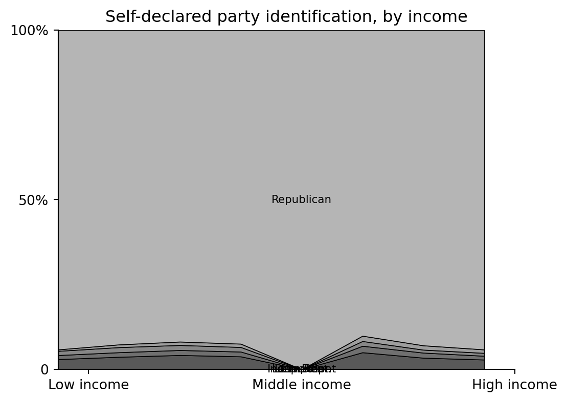
## Weighted cumulative profiles by income
The base-R plots use cumulative weighted proportions to draw stacked bands. The helper below mirrors `weighted.mean(indicator, weight, na.rm=TRUE)`.
```{python}
def weighted_mean_bool(mask, weights):
    ok = mask.notna() & weights.notna()
    if ok.sum() == 0 or weights[ok].sum() == 0:
        return np.nan
    return np.average(mask[ok].astype(float), weights=weights[ok])

def cumulative_profile(scores, n_scores, weights):
    out = np.empty((n_scores + 1, n_inc))
    out[-1, :] = 1.0
    for i in range(1, n_scores + 1):
        for j in range(1, n_inc + 1):
            out[i - 1, j - 1] = weighted_mean_bool((scores < i) & (inc == j), weights)
    return out

pid_profile = cumulative_profile(pid, 5, pop_weight0)
ideology_profile = cumulative_profile(ideology, 5, pop_weight0)

income_labels = income_order[:n_inc]
pd.DataFrame(pid_profile[:-1].T, columns=pid_label, index=income_labels).round(3).head()
```
```{python}
def draw_stacked_profile(profile, labels, title):
    x = np.arange(1, n_inc + 1)
    fig, ax = plt.subplots(figsize=(6, 4.5))
    grays = [str(0.35 + 0.09 * i) for i in range(len(labels))]
    for i, label in enumerate(labels):
        ax.fill_between(x, profile[i], profile[i + 1], color=grays[i], edgecolor="black", linewidth=0.6)
        center = n_inc // 2
        y = np.nanmean(profile[[i, i + 1], center])
        ax.text(x[center], y, label, ha="center", va="center", fontsize=8)
    ax.set(xlim=(1, n_inc), ylim=(0, 1), title=title)
    ax.set_xticks([1.5, 5, 8.5], ["Low income", "Middle income", "High income"])
    ax.set_yticks([0, 0.5, 1], ["0", "50%", "100%"])
    ax.spines[["top", "right"]].set_visible(False)
    return fig, ax

draw_stacked_profile(pid_profile, pid_label, "Self-declared party identification, by income")
```
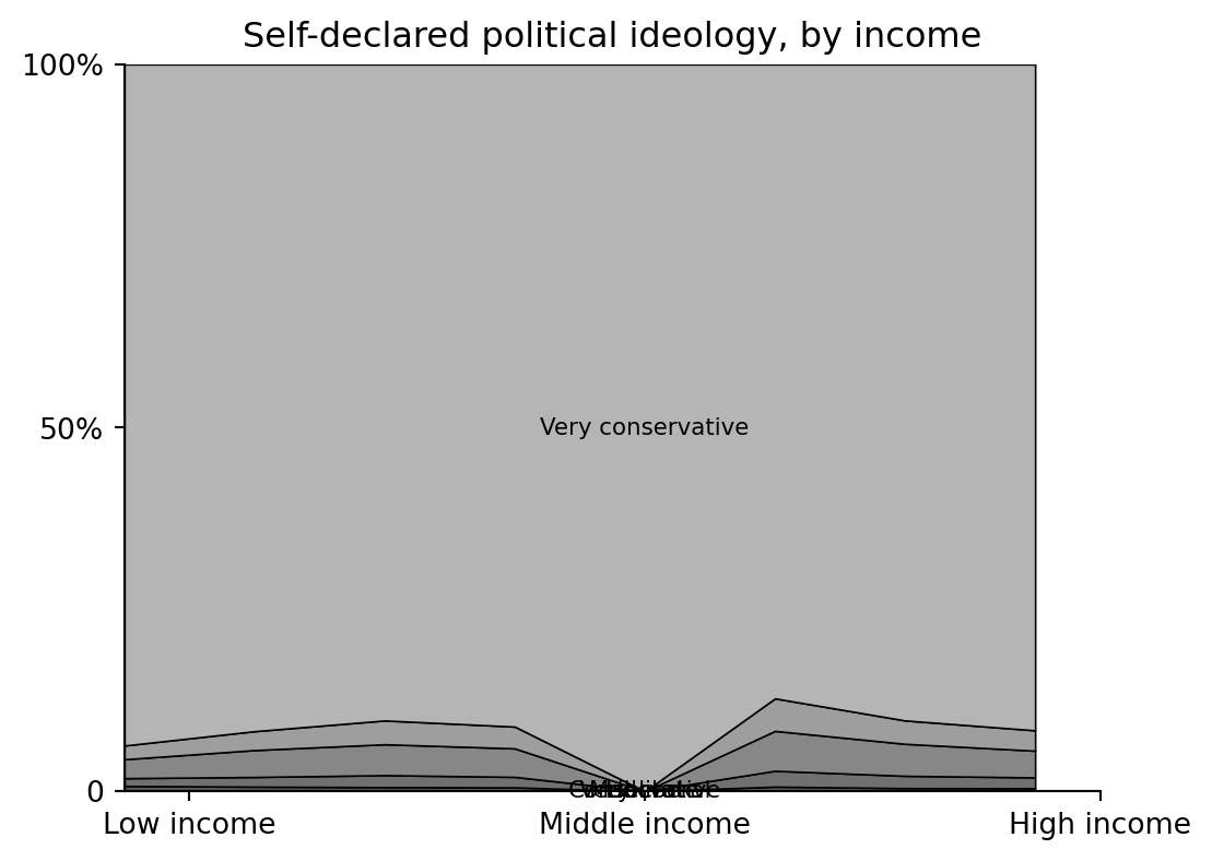
```{python}
draw_stacked_profile(ideology_profile, ideology_label, "Self-declared political ideology, by income")
```
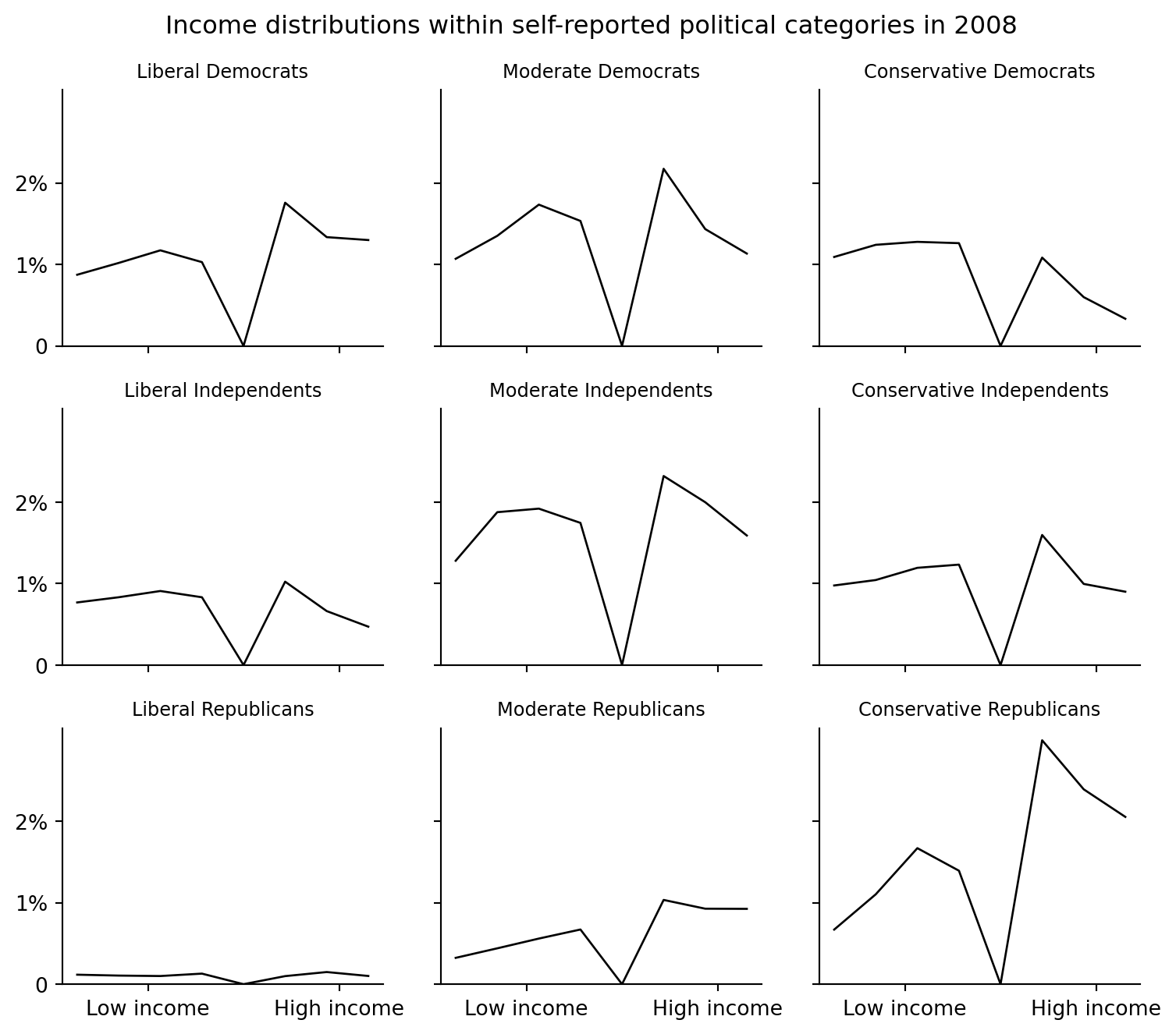
## Party-by-ideology income distributions
The final figure in the source groups respondents into three party categories and three ideology categories, then plots the weighted share of each combined category by income.
```{python}
pid2 = pd.Series(np.where(pid.eq(1), 1, np.where(pid.eq(5), 3, 2)), index=pew_pre.index)
ideology2 = pd.Series(np.where(ideology.isin([1, 2]), 1, np.where(ideology.eq(3), 2, 3)), index=pew_pre.index)
pid2_label = ["Democrats", "Independents", "Republicans"]
ideology2_label = ["Liberal", "Moderate", "Conservative"]

prop = np.empty((3, 3, n_inc))
for i in range(1, 4):
    for j in range(1, 4):
        for k in range(1, n_inc + 1):
            prop[i - 1, j - 1, k - 1] = weighted_mean_bool((pid2 == i) & (ideology2 == j) & (inc == k), pop_weight)

prop.round(4)[:, :, :3]
```
```{python}
fig, axes = plt.subplots(3, 3, figsize=(8, 7), sharex=True, sharey=True)
x = np.arange(1, n_inc + 1)
ymax = np.nanmax(prop)
for i in range(3):
    for j in range(3):
        ax = axes[i, j]
        ax.plot(x, prop[i, j, :], color="black", lw=1)
        ax.set_title(f"{ideology2_label[j]} {pid2_label[i]}", fontsize=9)
        ax.set_ylim(0, ymax * 1.05)
        ax.set_xticks([2.7, 7.3], ["Low income", "High income"])
        ax.set_yticks([0, 0.01, 0.02], ["0", "1%", "2%"])
        ax.spines[["top", "right"]].set_visible(False)
fig.suptitle("Income distributions within self-reported political categories in 2008")
fig.tight_layout()
```
## Religious attendance recode
The source also creates a five-level religious-attendance scale for later analyses. It is included here as a checked recode even though the displayed figures above do not use it.
```{python}
attend = norm_text(pew_pre["attend"])
relatt_map = {
    "never": 1,
    "seldom": 1,
    "a few times a year": 2,
    "once or twice a month": 3,
    "once a week": 4,
    "more than once a week": 5,
}
relatt = attend.map(relatt_map)
relatt_label = ["Nonattenders", "Rare attenders", "Occasional attenders", "Frequent attenders", "Very frequent church attenders"]
relatt.value_counts(dropna=False).sort_index()
```