# Beauty and teaching evaluations
Source: `Beauty/beauty.Rmd`
Hamermesh and Parker's teaching-evaluation data ask a deliberately simple regression question: do instructors rated as more beautiful also receive higher average teaching evaluations? The R original uses `rstanarm::stan_glm`; here the main computations are ordinary least squares in `statsmodels`, with a CmdStanPy template for the Bayesian analogue.
## Setup and data
```{python}
from pathlib import Path
import numpy as np
import pandas as pd
import matplotlib.pyplot as plt
import statsmodels.formula.api as smf

root = Path("../../ROS-Examples")
beauty = pd.read_csv(root / "Beauty/data/beauty.csv")
beauty.head()
```
```{python}
beauty.describe(include="all")
```
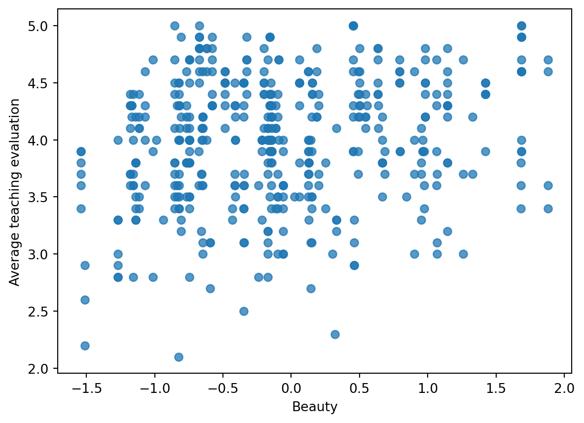
## Beauty as a single predictor
```{python}
fig, ax = plt.subplots()
ax.scatter(beauty["beauty"], beauty["eval"], alpha=0.75)
ax.set_xlabel("Beauty")
ax.set_ylabel("Average teaching evaluation")
```
```{python}
fit_1 = smf.ols("eval ~ beauty", data=beauty).fit()
fit_1.summary()
```
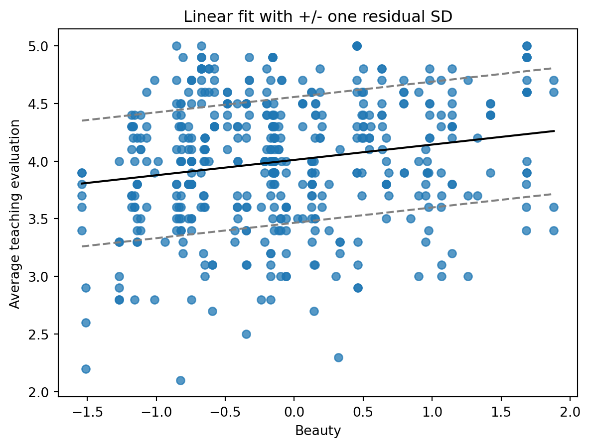
```{python}
xs = np.linspace(beauty.beauty.min(), beauty.beauty.max(), 200)
b0, b1 = fit_1.params["Intercept"], fit_1.params["beauty"]
sigma = np.sqrt(fit_1.mse_resid)

fig, ax = plt.subplots()
ax.scatter(beauty["beauty"], beauty["eval"], alpha=0.75)
ax.plot(xs, b0 + b1 * xs, color="black")
ax.plot(xs, b0 + b1 * xs + sigma, color="gray", linestyle="--")
ax.plot(xs, b0 + b1 * xs - sigma, color="gray", linestyle="--")
ax.set_xlabel("Beauty")
ax.set_ylabel("Average teaching evaluation")
ax.set_title("Linear fit with +/- one residual SD")
```
The slope is small on the evaluation scale, but positive in this simple regression.
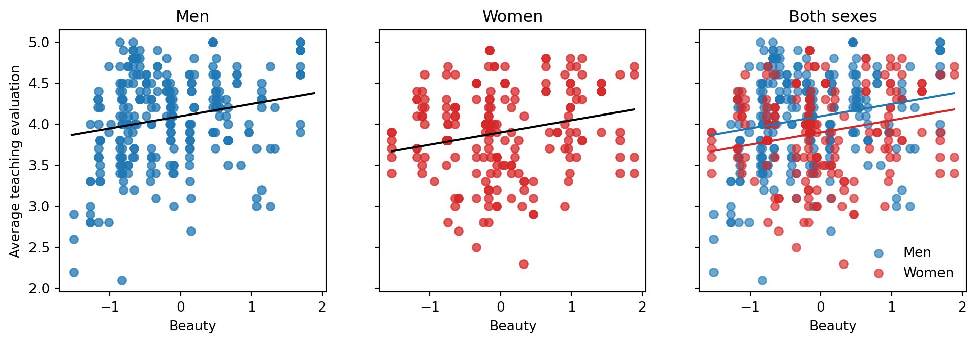
## Parallel lines for men and women
The R page next adds an indicator for women instructors. This gives two parallel regression lines: same beauty slope, different intercepts.
```{python}
fit_2 = smf.ols("eval ~ beauty + female", data=beauty).fit()
fit_2.summary()
```
```{python}
def line_parallel(x, female):
    p = fit_2.params
    return p["Intercept"] + p["beauty"] * x + p["female"] * female

fig, axes = plt.subplots(1, 3, figsize=(12, 3.5), sharex=True, sharey=True)
for ax, female, title, color in [(axes[0], 0, "Men", "tab:blue"), (axes[1], 1, "Women", "tab:red")]:
    d = beauty[beauty.female == female]
    ax.scatter(d.beauty, d["eval"], alpha=0.75, color=color)
    ax.plot(xs, line_parallel(xs, female), color="black")
    ax.set_title(title)
    ax.set_xlabel("Beauty")
axes[0].set_ylabel("Average teaching evaluation")

axes[2].scatter(beauty.loc[beauty.female == 0, "beauty"], beauty.loc[beauty.female == 0, "eval"], color="tab:blue", alpha=0.65, label="Men")
axes[2].scatter(beauty.loc[beauty.female == 1, "beauty"], beauty.loc[beauty.female == 1, "eval"], color="tab:red", alpha=0.65, label="Women")
axes[2].plot(xs, line_parallel(xs, 0), color="tab:blue")
axes[2].plot(xs, line_parallel(xs, 1), color="tab:red")
axes[2].set_title("Both sexes")
axes[2].set_xlabel("Beauty")
axes[2].legend(frameon=False)
```
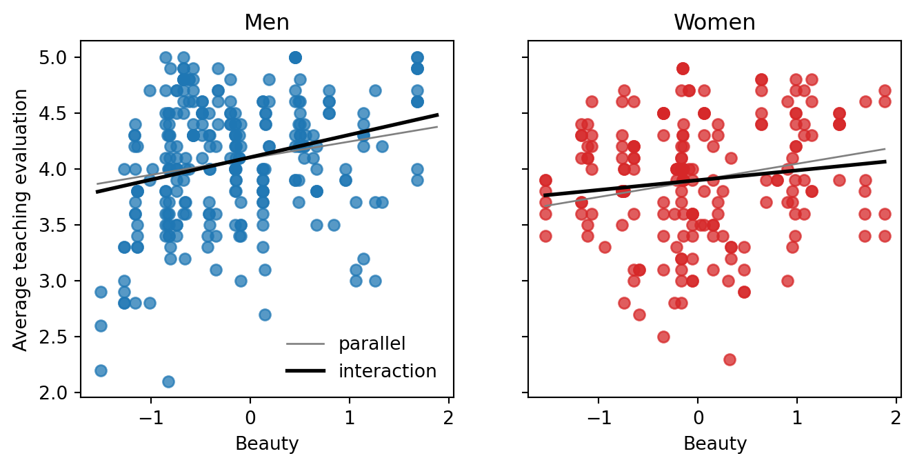
## Allow the beauty slope to differ by sex
```{python}
fit_3 = smf.ols("eval ~ beauty * female", data=beauty).fit()
fit_3.summary()
```
```{python}
def line_interaction(x, female):
    p = fit_3.params
    return (
        p["Intercept"]
        + p["beauty"] * x
        + p["female"] * female
        + p["beauty:female"] * x * female
    )

fig, axes = plt.subplots(1, 2, figsize=(8, 3.5), sharex=True, sharey=True)
for ax, female, title, color in [(axes[0], 0, "Men", "tab:blue"), (axes[1], 1, "Women", "tab:red")]:
    d = beauty[beauty.female == female]
    ax.scatter(d.beauty, d["eval"], alpha=0.75, color=color)
    ax.plot(xs, line_parallel(xs, female), color="gray", linewidth=1, label="parallel")
    ax.plot(xs, line_interaction(xs, female), color="black", linewidth=2, label="interaction")
    ax.set_title(title)
    ax.set_xlabel("Beauty")
axes[0].set_ylabel("Average teaching evaluation")
axes[0].legend(frameon=False)
```
## Additional controls
The original page fits a sequence of regressions with age, minority status, non-English indicator, lower-division course indicator, and course fixed effects. `statsmodels` formula notation mirrors the R formulas closely.
```{python}
formulas = {
    "beauty + female + age": "eval ~ beauty + female + age",
    "beauty + female + minority": "eval ~ beauty + female + minority",
    "beauty + female + nonenglish": "eval ~ beauty + female + nonenglish",
    "beauty + female + nonenglish + lower": "eval ~ beauty + female + nonenglish + lower",
    "beauty + course indicators": "eval ~ beauty + C(course_id)",
}

rows = []
for label, formula in formulas.items():
    m = smf.ols(formula, data=beauty).fit()
    rows.append({
        "model": label,
        "beauty_coef": m.params.get("beauty", np.nan),
        "beauty_se": m.bse.get("beauty", np.nan),
        "n": int(m.nobs),
        "r2": m.rsquared,
    })
pd.DataFrame(rows)
```
## CmdStanPy version of `stan_glm(eval ~ beauty)`
```{python}
#| eval: false
from cmdstanpy import CmdStanModel

stan_code = """
data {
  int<lower=1> N;
  vector[N] x;
  vector[N] y;
}
parameters {
  real alpha;
  real beta;
  real<lower=0> sigma;
}
model {
  alpha ~ normal(0, 10);
  beta ~ normal(0, 10);
  sigma ~ exponential(1);
  y ~ normal(alpha + beta * x, sigma);
}
generated quantities {
  vector[N] y_rep;
  for (n in 1:N) y_rep[n] = normal_rng(alpha + beta * x[n], sigma);
}
"""
Path("beauty_lm.stan").write_text(stan_code)
model = CmdStanModel(stan_file="beauty_lm.stan")
fit = model.sample(
    data={"N": len(beauty), "x": beauty.beauty.to_numpy(), "y": beauty["eval"].to_numpy()},
    chains=4,
    seed=123,
)
fit.summary().loc[["alpha", "beta", "sigma"]]
```