Simple regression with weak Bayesian regularization

Source: Simplest/simplest.Rmd

This is the Bayesian companion to the least-squares “simplest” example. The original R page uses rstanarm::stan_glm; here we show the same simulated comparisons with statsmodels for the point estimates and a small CmdStanPy model for posterior draws when desired.

Setup and simulated data

from pathlib import Path
import numpy as np
import pandas as pd
import matplotlib.pyplot as plt
import statsmodels.api as sm

rng = np.random.default_rng(2141)
root = Path("../../ROS-Examples")

x = np.arange(1, 21)
a = 0.2
b = 0.3
sigma = 0.5
y = a + b * x + sigma * rng.normal(size=len(x))
fake = pd.DataFrame({"x": x, "y": y})

fit_ols = sm.OLS(fake["y"], sm.add_constant(fake["x"])).fit()
fit_ols.params

const    0.251307
x        0.299993
dtype: float64

a_hat, b_hat = fit_ols.params["const"], fit_ols.params["x"]
fig, ax = plt.subplots(figsize=(6, 4.4))
ax.scatter(fake.x, fake.y, color="black", s=25)
ax.plot(fake.x, a_hat + b_hat * fake.x, color="black")
ax.text(fake.x.mean(), a_hat + b_hat * fake.x.mean() - 0.2, f"   y = {a_hat:.2f} + {b_hat:.2f} x")
ax.set(title="Data and fitted regression line", xlabel="x", ylabel="y")
ax.spines[["top", "right"]].set_visible(False)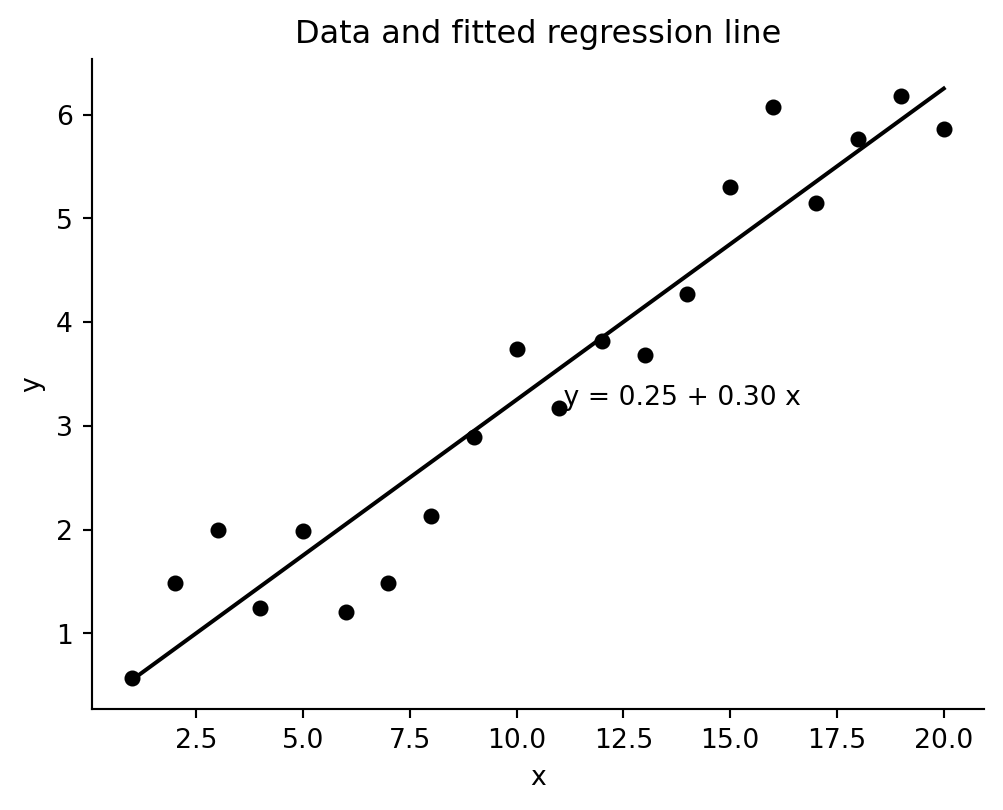

A direct Stan model for the same regression

The R code calls stan_glm(y ~ x). A minimal equivalent model is useful because it exposes the likelihood and priors explicitly. The priors below are deliberately weak relative to the simulated data scale.

from cmdstanpy import CmdStanModel

stan_code = """
data {
  int<lower=1> N;
  vector[N] x;
  vector[N] y;
}
parameters {
  real alpha;
  real beta;
  real<lower=0> sigma;
}
model {
  alpha ~ normal(0, 10);
  beta ~ normal(0, 10);
  sigma ~ exponential(1);
  y ~ normal(alpha + beta * x, sigma);
}
"""
stan_file = Path("_generated/simple_regression.stan")
stan_file.parent.mkdir(exist_ok=True)
stan_file.write_text(stan_code)

model = CmdStanModel(stan_file=str(stan_file))
stan_data = {"N": len(fake), "x": fake.x.to_numpy(), "y": fake.y.to_numpy()}
fit_stan = model.sample(data=stan_data, seed=2141, chains=4, parallel_chains=4, show_progress=False)
draws = fit_stan.draws_pd()
draws[["alpha", "beta", "sigma"]].describe(percentiles=[0.05, 0.5, 0.95])

	alpha	beta	sigma
count	4000.000000	4000.000000	4000.000000
mean	0.248009	0.300297	0.568105
std	0.262963	0.022037	0.106309
min	-0.723648	0.197527	0.321306
5%	-0.177646	0.264021	0.427331
50%	0.243569	0.300482	0.553648
95%	0.677876	0.335236	0.763470
max	1.502440	0.398738	1.154650

fig, ax = plt.subplots(figsize=(6, 4.4))
ax.scatter(fake.x, fake.y, color="black", s=25)
xx = np.linspace(fake.x.min(), fake.x.max(), 100)
for _, row in draws.sample(30, random_state=2141).iterrows():
    ax.plot(xx, row["alpha"] + row["beta"] * xx, color="0.6", lw=0.6, alpha=0.7)
ax.plot(xx, draws["alpha"].median() + draws["beta"].median() * xx, color="black", lw=1.5)
ax.set(title="Posterior regression lines", xlabel="x", ylabel="y")
ax.spines[["top", "right"]].set_visible(False)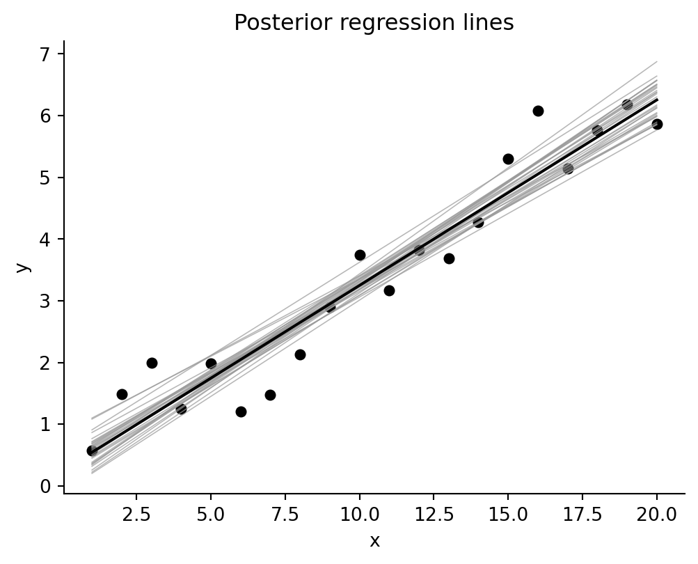

A mean as a one-parameter regression

Estimating a population mean is a regression with only an intercept. The original page fits this with stan_glm(y_0 ~ 1); the table compares direct and regression calculations.

rng = np.random.default_rng(2141)
n_0 = 200
y_0 = rng.normal(2.0, 5.0, size=n_0)
fit_mean = sm.OLS(y_0, np.ones((n_0, 1))).fit()

pd.DataFrame(
    {
        "mean": [y_0.mean()],
        "ols_intercept": [fit_mean.params[0]],
        "se_mean": [y_0.std(ddof=1) / np.sqrt(n_0)],
        "ols_se": [fit_mean.bse[0]],
    }
)

	mean	ols_intercept	se_mean	ols_se
0	2.01524	2.01524	0.347483	0.347483

A difference as a regression slope

A two-group comparison is a regression on an intercept and an indicator. The intercept is the mean of the baseline group and the slope is the difference between group means.

rng = np.random.default_rng(2141)
n_1 = 300
y_1 = rng.normal(8.0, 5.0, size=n_1)

y = np.r_[y_0, y_1]
x = np.r_[np.zeros(n_0), np.ones(n_1)]
fake_groups = pd.DataFrame({"y": y, "x": x})
fit_groups = sm.OLS(fake_groups["y"], sm.add_constant(fake_groups["x"])).fit()

pd.DataFrame(
    {
        "mean_0": [y_0.mean()],
        "mean_1": [y_1.mean()],
        "difference": [y_1.mean() - y_0.mean()],
        "regression_intercept": [fit_groups.params["const"]],
        "regression_slope": [fit_groups.params["x"]],
    }
)

	mean_0	mean_1	difference	regression_intercept	regression_slope
0	2.01524	8.252959	6.237719	2.01524	6.237719

fig, ax = plt.subplots(figsize=(5.6, 4.5))
ax.scatter(x, y, color="black", s=10, alpha=0.45)
ax.set_xticks([0, 1])
ax.axhline(y_0.mean(), color="0.5", ls="--", lw=1)
ax.axhline(y_1.mean(), color="0.5", ls="--", lw=1)
ax.plot([0, 1], fit_groups.params["const"] + fit_groups.params["x"] * np.array([0, 1]), color="black")
ax.text(0.48, fit_groups.params["const"] + 0.5 * fit_groups.params["x"] - 1, f"y = {fit_groups.params['const']:.2f} + {fit_groups.params['x']:.2f} x")
ax.set(title="Regression on an indicator is a difference in means", xlabel="Indicator, x", ylabel="y")
ax.spines[["top", "right"]].set_visible(False)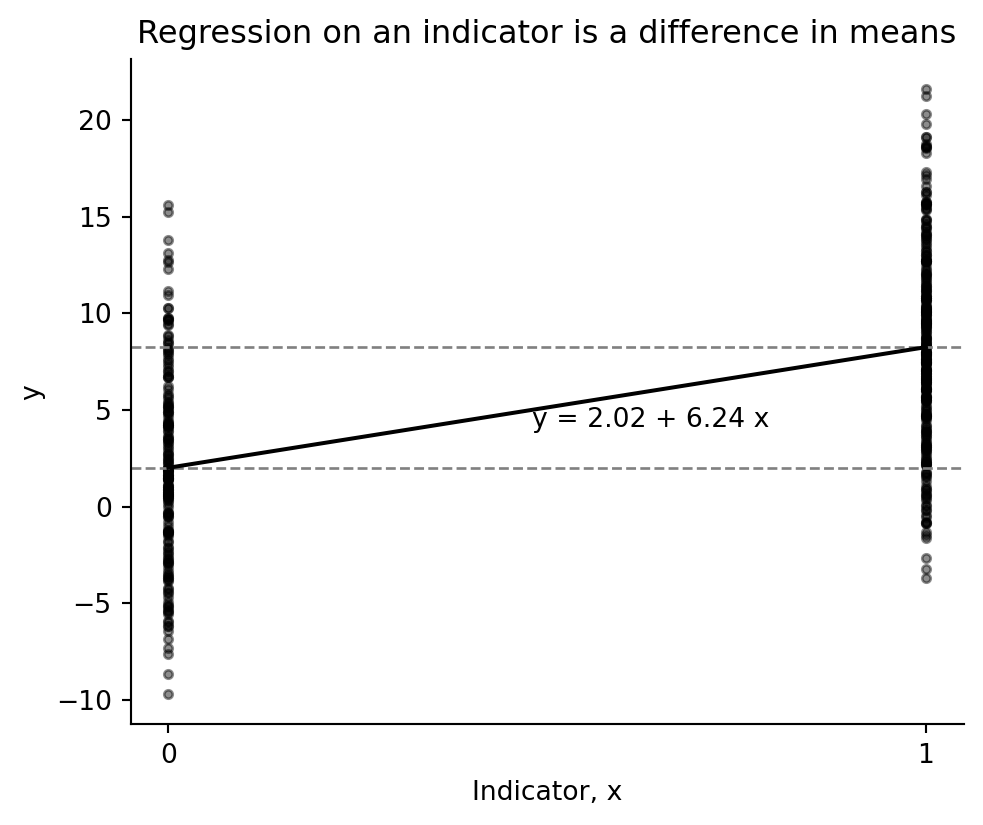

Flat-prior interpretation

With a Gaussian likelihood and flat priors on the coefficients and scale, the posterior mode for the regression coefficients is the least-squares estimate. This is the Python analogue of the final stan_glm(..., prior=NULL, prior_intercept=NULL, prior_aux=NULL) call in the R page.