Simplest linear regressions

Source: Simplest/simplest_lm.Rmd

This page keeps the linear-regression examples but fits them with the same lapylace Gaussian path used elsewhere in the book.

Simulated regression

from pathlib import Path
import numpy as np
import pandas as pd
import matplotlib.pyplot as plt
import lapylace as lp

root = Path("../../ROS-Examples")

def coef_medians(fit):
    return pd.Series(
        [np.median(fit.alpha_draws()), *np.median(fit.beta_draws(), axis=0)],
        index=["Intercept", *fit.columns],
    )

def fit_glm(formula, data, family=None, seed=1, prior_scale=2.5, intercept_scale=5, aux_scale=10, **kwargs):
    return lp.stan_glm(
        formula,
        data=data,
        family=family or lp.gaussian(),
        prior=lp.normal(0, prior_scale),
        prior_intercept=lp.normal(0, intercept_scale),
        prior_aux=lp.exponential(aux_scale),
        chains=2,
        parallel_chains=2,
        iter_warmup=300,
        iter_sampling=500,
        seed=seed,
        refresh=100,
        **kwargs,
    )

rng = np.random.default_rng(18801)
fake = pd.DataFrame({"x": rng.normal(size=100)})
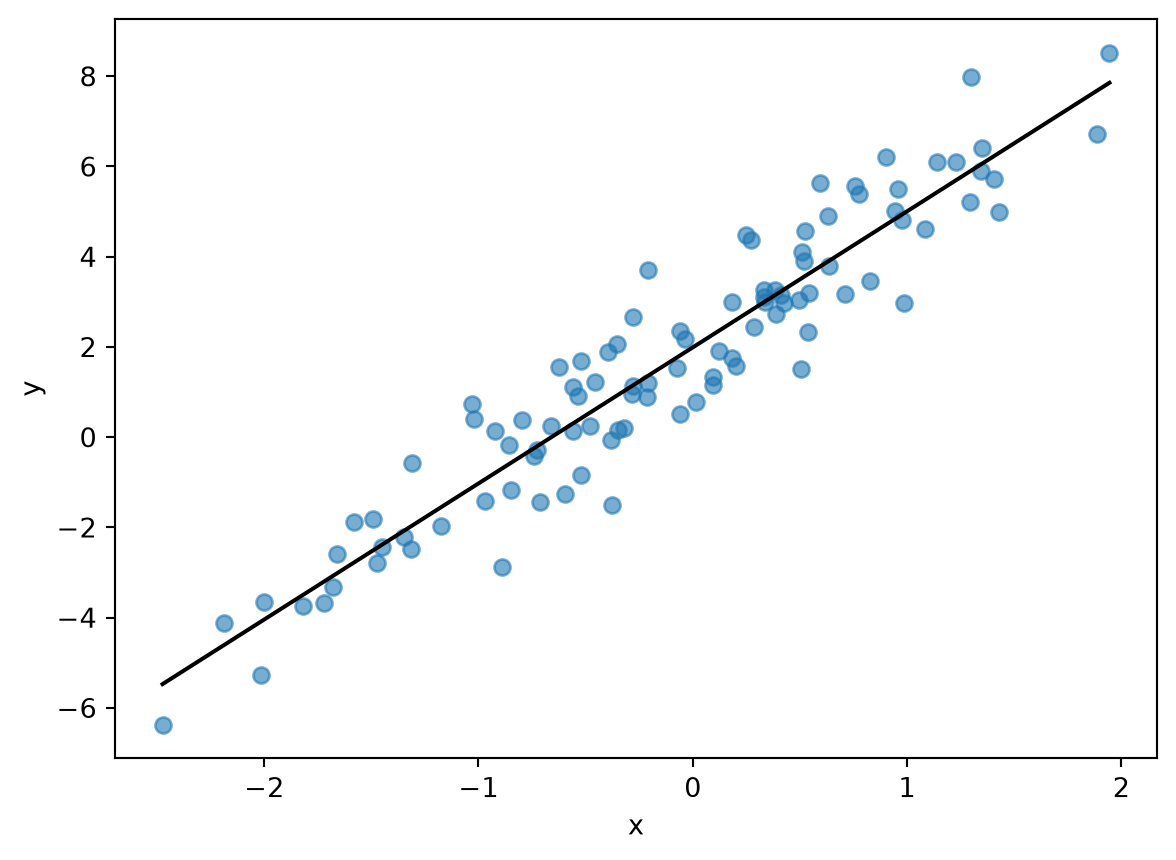
fake["y"] = 2 + 3*fake.x + rng.normal(0, 1, size=len(fake))
fit = fit_glm("y ~ x", fake, seed=18802, prior_scale=5, intercept_scale=5, aux_scale=2)
fit.summary(["alpha", "beta", "sigma"])

	Mean	MCSE	StdDev	5%	50%	95%	N_Eff	N_Eff/s	R_hat
alpha	1.98822	0.003718	0.098752	1.82202	1.98843	2.14757	705.57200	16035.70000	0.999246
beta[1]	3.01627	0.003689	0.105777	2.83968	3.01355	3.19338	822.35100	18689.80000	1.001660
sigma	0.99280	0.002470	0.072270	0.87743	0.99094	1.11223	858.09649	19502.19304	1.002770

grid = pd.DataFrame({"x": np.linspace(fake.x.min(), fake.x.max(), 100)})
pred = fit.posterior_epred(grid)
fig, ax = plt.subplots()
ax.scatter(fake.x, fake.y, alpha=.6)
ax.plot(grid.x, pred.mean(axis=0), color="black")
ax.set_xlabel("x")
ax.set_ylabel("y")

Text(0, 0.5, 'y')