Code
import numpy as np
import pandas as pd
import matplotlib.pyplot as plt

rng = np.random.default_rng(20260531)Source: ProbabilitySimulation/probsim.Rmd
This example translates the chapter’s probability-model simulations directly into NumPy. The goal is to make the random variables visible: binomial births, mixtures induced by twin births, common discrete and continuous distributions, and repeated sampling of adult heights.
import numpy as np
import pandas as pd
import matplotlib.pyplot as plt
rng = np.random.default_rng(20260531)p_girl_single = 0.488
n_births = 400
one_draw = rng.binomial(n_births, p_girl_single)
one_draw211Repeating the same experiment gives the sampling distribution for the number of girls.
n_sims = 1_000
girls_simple = rng.binomial(n_births, p_girl_single, size=n_sims)

pd.Series(girls_simple).describe(percentiles=[0.05, 0.5, 0.95])
count 1000.000000
mean 195.022000
std 9.736031
min 165.000000
5% 180.000000
50% 195.000000
95% 211.000000
max 227.000000
dtype: float64fig, ax = plt.subplots(figsize=(6, 3.5))
ax.hist(girls_simple, bins=np.arange(150, 251, 5), color="0.75", edgecolor="white")
ax.set_xlabel("girls in 400 births")
ax.set_ylabel("simulation count")
ax.set_title("Binomial simulation: n=400, p=0.488")Text(0.5, 1.0, 'Binomial simulation: n=400, p=0.488')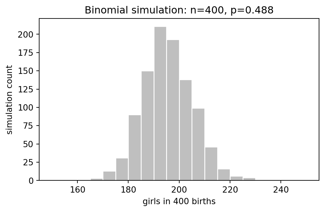
The R example then lets each recorded birth event be a single birth, an identical-twin birth, or a fraternal-twin birth. Identical twins share sex, while fraternal twins are modeled as two independent Bernoulli draws.
def simulate_girls_with_twins(rng, n_events=400):
    birth_type = rng.choice(
        ["fraternal twin", "identical twin", "single birth"],
        size=n_events,
        p=[1/125, 1/300, 1 - 1/125 - 1/300],
    )
    girls = np.empty(n_events, dtype=int)
    single = birth_type == "single birth"
    identical = birth_type == "identical twin"
    fraternal = birth_type == "fraternal twin"
    girls[single] = rng.binomial(1, 0.488, size=single.sum())
    girls[identical] = 2 * rng.binomial(1, 0.495, size=identical.sum())
    girls[fraternal] = rng.binomial(2, 0.495, size=fraternal.sum())
    return girls.sum(), pd.Series(birth_type).value_counts()

girls_once, type_counts = simulate_girls_with_twins(rng)
girls_once, type_counts
(np.int64(191),
single birth 388
fraternal twin 9
identical twin 3
Name: count, dtype: int64)girls_twins = np.array([simulate_girls_with_twins(rng)[0] for _ in range(n_sims)])
summary = pd.DataFrame({
"simple binomial": pd.Series(girls_simple).describe(),
"with twins": pd.Series(girls_twins).describe(),
})
summary| simple binomial | with twins | |
|---|---|---|
| count | 1000.000000 | 1000.000000 |
| mean | 195.022000 | 197.913000 |
| std | 9.736031 | 9.834233 |
| min | 165.000000 | 168.000000 |
| 25% | 189.000000 | 191.000000 |
| 50% | 195.000000 | 198.000000 |
| 75% | 202.000000 | 205.000000 |
| max | 227.000000 | 226.000000 |
fig, ax = plt.subplots(figsize=(6, 3.5))
ax.hist(girls_twins, bins=np.arange(150, 251, 5), color="0.70", edgecolor="white")
ax.set_xlabel("girls among 400 birth events")
ax.set_ylabel("simulation count")
ax.set_title("Simulation with single and twin births")
Text(0.5, 1.0, 'Simulation with single and twin births')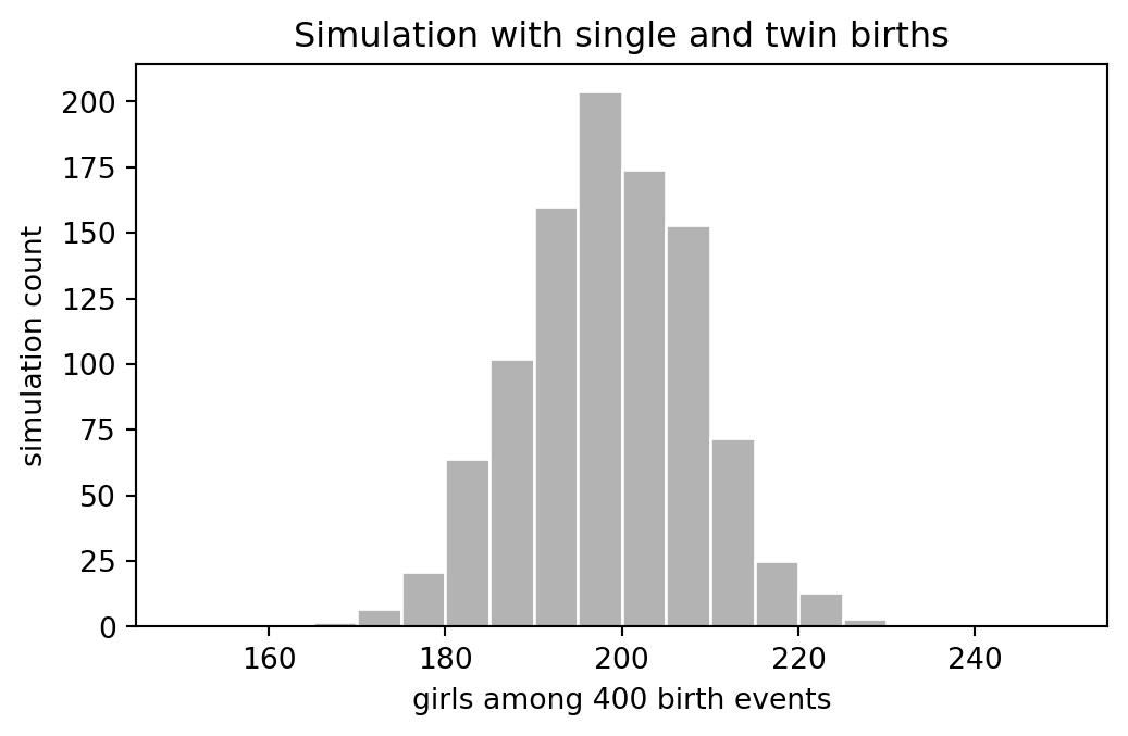
y1 = rng.normal(3, 0.5, size=n_sims)
y2 = np.exp(y1)
y3 = rng.binomial(20, 0.6, size=n_sims)
y4 = rng.poisson(5, size=n_sims)fig, axs = plt.subplots(2, 2, figsize=(9, 6))
axs = axs.ravel()
axs[0].hist(y1, bins=np.arange(np.floor(y1.min()), np.ceil(y1.max()) + 0.2, 0.2), edgecolor="white")
axs[0].set_title("Normal(3, 0.5)")
axs[1].hist(y2, bins=np.arange(0, np.ceil(y2.max()) + 5, 5), edgecolor="white")
axs[1].set_title("exp(normal): lognormal")
axs[2].hist(y3, bins=np.arange(-0.5, 21.5, 1), edgecolor="white")
axs[2].set_title("Binomial(20, 0.6)")
axs[3].hist(y4, bins=np.arange(-0.5, y4.max() + 1.5, 1), edgecolor="white")
axs[3].set_title("Poisson(5)")
fig.tight_layout()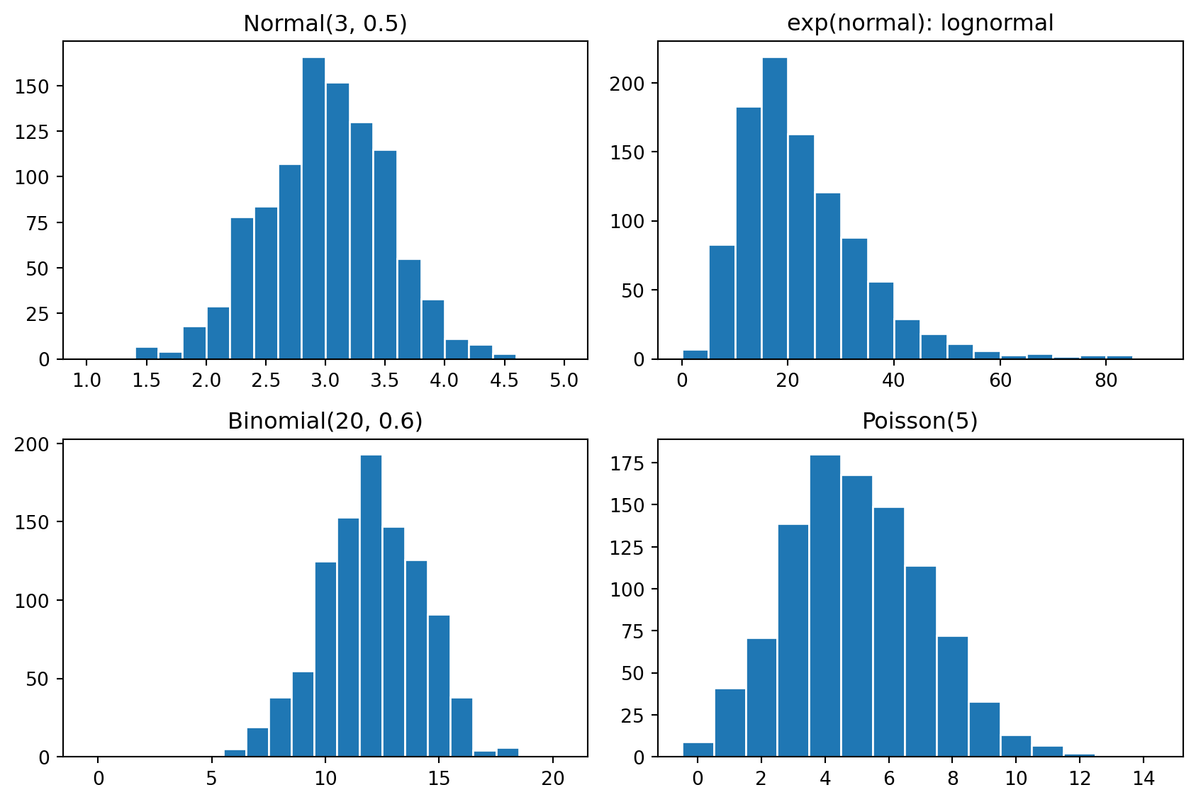
Adult height is simulated by first drawing sex and then drawing height from the corresponding sex-specific normal distribution.
def sample_adult_heights(rng, n):
    male = rng.binomial(1, 0.48, size=n).astype(bool)
    height = np.empty(n)
    height[male] = rng.normal(69.1, 2.9, size=male.sum())
    height[~male] = rng.normal(64.5, 2.7, size=(~male).sum())
    return height

sample_adult_heights(rng, 1)[0]np.float64(66.14244539104533)N = 10
heights = sample_adult_heights(rng, N)
heights.mean()np.float64(65.53642411360696)avg_height = np.array([sample_adult_heights(rng, N).mean() for _ in range(n_sims)])
max_height = np.array([sample_adult_heights(rng, N).max() for _ in range(n_sims)])
pd.DataFrame({"average height": avg_height, "maximum height": max_height}).describe(percentiles=[0.05, 0.5, 0.95])| average height | maximum height | |
|---|---|---|
| count | 1000.000000 | 1000.000000 |
| mean | 66.681949 | 72.361921 |
| std | 1.134083 | 1.927259 |
| min | 62.650524 | 66.618626 |
| 5% | 64.860539 | 69.454894 |
| 50% | 66.659145 | 72.314885 |
| 95% | 68.576982 | 75.670772 |
| max | 70.156175 | 80.132245 |
fig, axs = plt.subplots(1, 2, figsize=(9, 3.5))
axs[0].hist(avg_height, bins=30, edgecolor="white")
axs[0].set_title("Average height of 10 adults")
axs[1].hist(max_height, bins=30, edgecolor="white")
axs[1].set_title("Maximum height among 10 adults")
for ax in axs:
    ax.set_xlabel("height (inches)")
    ax.set_ylabel("simulation count")
fig.tight_layout()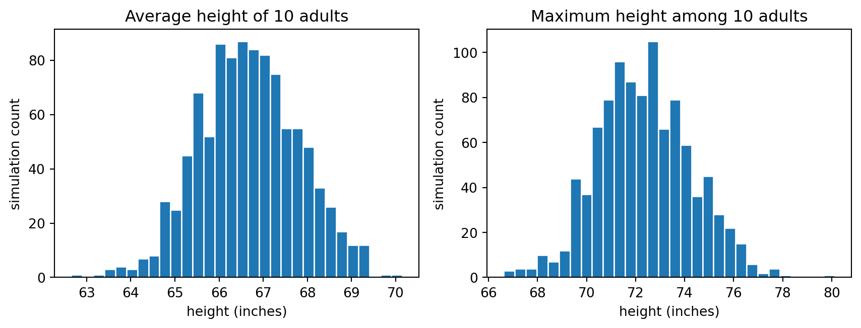
The maximum has a much more right-shifted distribution than the average, even though both are generated from the same underlying adult-height mixture.