Simple causal regression graphics

Source: SimpleCausal/causal.Rmd

These simulations show how a regression slope can be interpreted as a treatment contrast in simple randomized settings, and why straight-line summaries can mislead for nonlinear treatment response.

import numpy as np
import pandas as pd
import matplotlib.pyplot as plt
import statsmodels.formula.api as smf

rng = np.random.default_rng(1151)

Linear treatment response

N = 50
x = rng.uniform(1, 5, N)
y = rng.normal(10 + 3*x, 3)
x_binary = (x >= 3).astype(int)
data = pd.DataFrame({"x": x, "y": y, "x_binary": x_binary})
fit_bin = smf.ols("y ~ x_binary", data=data).fit()
fit_cont = smf.ols("y ~ x", data=data).fit()
fit_bin.params, fit_cont.params

(Intercept    16.299469
 x_binary      5.344403
 dtype: float64,
 Intercept    10.871194
 x             2.792726
 dtype: float64)

fig, axs = plt.subplots(1, 2, figsize=(10, 4))
axs[0].scatter(x_binary, y, s=18, color="black")
axs[0].plot([0, 1], fit_bin.params["Intercept"] + fit_bin.params["x_binary"]*np.array([0,1]), color="black")
axs[0].set_xticks([0, 1], ["Control", "Treatment"])
axs[0].set_ylabel("Outcome measurement")
axs[0].set_title("Binary treatment")
xs = np.linspace(1, 5, 100)
axs[1].scatter(x, y, s=18, color="black")
axs[1].plot(xs, fit_cont.params["Intercept"] + fit_cont.params["x"]*xs, color="black")
axs[1].set_xlabel("Treatment level")
axs[1].set_title("Continuous treatment")

Text(0.5, 1.0, 'Continuous treatment')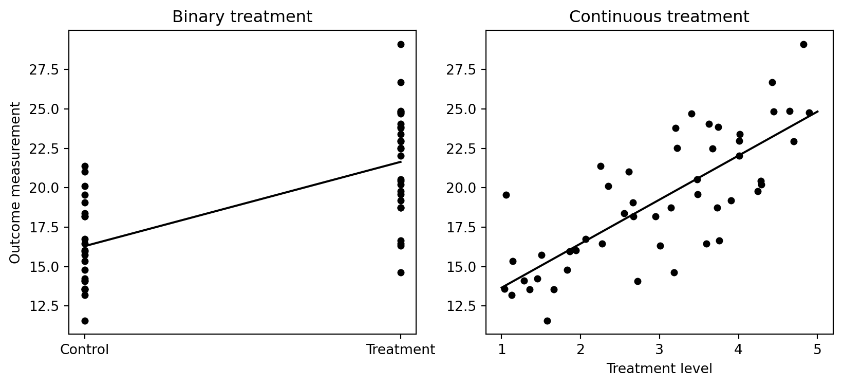

Nonlinear response approximated with a line

y2 = rng.normal(5 + 30*np.exp(-x), 2)
data2 = pd.DataFrame({"x": x, "y": y2})
fit_nl = smf.ols("y ~ x", data=data2).fit()
fig, axs = plt.subplots(1, 2, figsize=(10, 4))
for ax in axs:
    ax.scatter(x, y2, s=18, color="black")
    ax.set_xlabel("Treatment level")
xs = np.linspace(1, 5, 100)
axs[0].plot(xs, 5 + 30*np.exp(-xs), color="black")
axs[0].set_title("Nonlinear treatment effect")
axs[1].plot(xs, fit_nl.params["Intercept"] + fit_nl.params["x"]*xs, color="black")
axs[1].set_title("Straight-line approximation")

Text(0.5, 1.0, 'Straight-line approximation')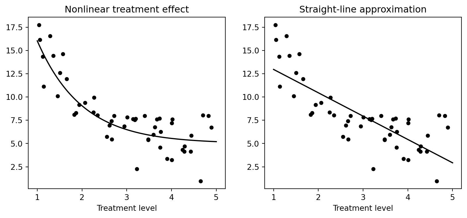

Pre-treatment predictor plus treatment indicator

N = 100
z = np.repeat([0, 1], N//2)
xx = np.where(z == 0, rng.normal(0, 1.2, N)**2, rng.normal(0, .8, N)**2)
yy = rng.normal(20 + 5*xx + 10*z, 3)
d3 = pd.DataFrame({"xx": xx, "z": z, "yy": yy})
fit_adj = smf.ols("yy ~ xx + z", data=d3).fit()
fit_adj.params

Intercept    19.127654
xx            5.230688
z            11.078474
dtype: float64

fig, ax = plt.subplots(figsize=(6, 4))
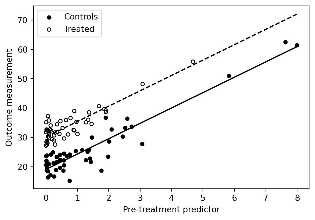
ax.scatter(xx[z==0], yy[z==0], s=18, color="black", label="Controls")
ax.scatter(xx[z==1], yy[z==1], s=18, facecolors="none", edgecolors="black", label="Treated")
xs = np.linspace(0, xx.max(), 100)
ax.plot(xs, fit_adj.params["Intercept"] + fit_adj.params["xx"]*xs, color="black")
ax.plot(xs, fit_adj.params["Intercept"] + fit_adj.params["z"] + fit_adj.params["xx"]*xs, color="black", linestyle="--")
ax.set_xlabel("Pre-treatment predictor")
ax.set_ylabel("Outcome measurement")
ax.legend()