# Arsenic wells: building logistic regression models
Source: `Arsenic/arsenic_logistic_building.Rmd`
This ports the core model-building sequence for the Bangladesh wells example.
## Load data
```{python}
from pathlib import Path
import numpy as np
import pandas as pd
import matplotlib.pyplot as plt
import lapylace as lp
from scipy.special import expit

root = Path("../../ROS-Examples")
wells = pd.read_csv(root / "Arsenic/data/wells.csv")
wells["dist100"] = wells["dist"] / 100
wells.head()
```
```{python}
def coef_medians(fit):
    return pd.Series(
        [np.median(fit.alpha_draws()), *np.median(fit.beta_draws(), axis=0)],
        index=["Intercept", *fit.columns],
    )
```
## Null-model log scores
```{python}
y = wells["switch"].to_numpy()
for p in [0.5, y.mean()]:
    log_score = np.sum(y*np.log(p) + (1-y)*np.log(1-p))
    print(round(p, 3), round(log_score, 1))
```
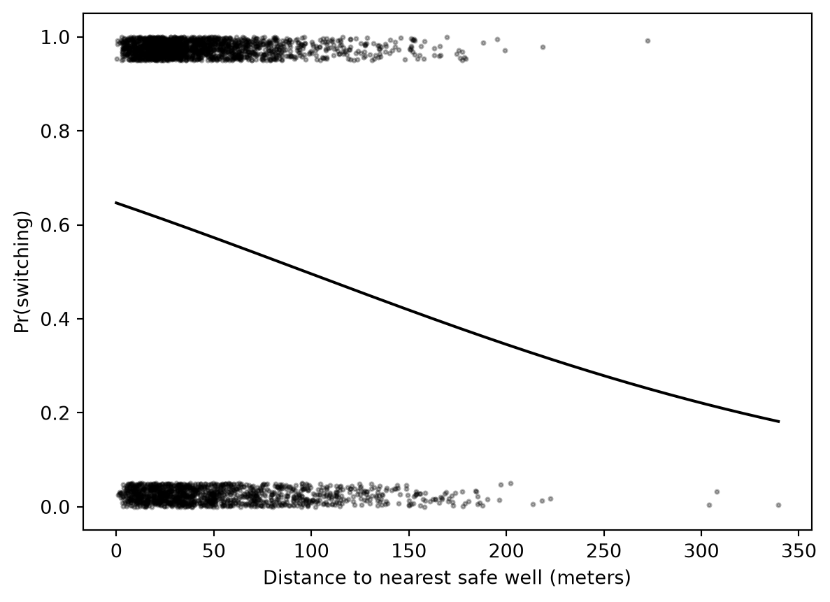
## Single predictor: distance
R original:
```r
stan_glm(switch ~ dist100, family = binomial(link = "logit"), data=wells)
```
Python uses the same formula-first Bayesian GLM path through `lapylace`:
```{python}
fit_2 = lp.stan_glm(
    "switch ~ dist100",
    data=wells,
    family=lp.bernoulli(),
    prior=lp.normal(0, 2.5),
    prior_intercept=lp.normal(0, 5),
    chains=4,
    parallel_chains=4,
    iter_warmup=500,
    iter_sampling=1000,
    seed=15101,
    refresh=100,
)
coef_2 = coef_medians(fit_2)
coef_2.round(2)
```
```{python}
fig, ax = plt.subplots()
rng = np.random.default_rng(123)
y_jit = y + (1 - 2*y) * rng.uniform(0, 0.05, size=len(y))
ax.scatter(wells["dist"], y_jit, s=4, color="black", alpha=0.3)
xs = np.linspace(0, wells["dist"].max(), 300)
ax.plot(xs, expit(coef_2["Intercept"] + coef_2["dist100"] * xs/100), color="black")
ax.set_xlabel("Distance to nearest safe well (meters)")
ax.set_ylabel("Pr(switching)")
```
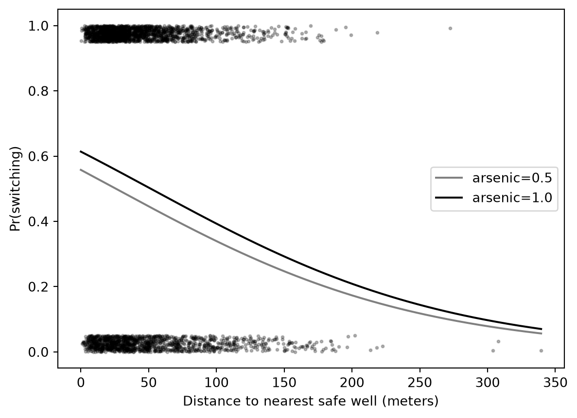
## Two predictors: distance + arsenic
```{python}
fit_3 = lp.stan_glm(
    "switch ~ dist100 + arsenic",
    data=wells,
    family=lp.bernoulli(),
    prior=lp.normal(0, 2.5),
    prior_intercept=lp.normal(0, 5),
    chains=4,
    parallel_chains=4,
    iter_warmup=500,
    iter_sampling=1000,
    seed=15102,
    refresh=100,
)
coef_3 = coef_medians(fit_3)
coef_3.round(2)
```
Compare predicted curves at fixed arsenic levels:
```{python}
fig, ax = plt.subplots()
ax.scatter(wells["dist"], y_jit, s=4, color="black", alpha=0.25)
for a, color in [(0.5, "gray"), (1.0, "black")]:
    p = expit(coef_3["Intercept"] + coef_3["dist100"]*xs/100 + coef_3["arsenic"]*a)
    ax.plot(xs, p, color=color, label=f"arsenic={a}")
ax.legend()
ax.set_xlabel("Distance to nearest safe well (meters)")
ax.set_ylabel("Pr(switching)")
```
## Interaction
```{python}
fit_4 = lp.stan_glm(
    "switch ~ dist100 * arsenic",
    data=wells,
    family=lp.bernoulli(),
    prior=lp.normal(0, 2.5),
    prior_intercept=lp.normal(0, 5),
    chains=4,
    parallel_chains=4,
    iter_warmup=500,
    iter_sampling=1000,
    seed=15103,
    refresh=100,
)
coef_4 = coef_medians(fit_4)
coef_4.round(2)
```
## CmdStanPy equivalent
`lapylace` generates the Bernoulli-logit Stan model behind the formula call:
```stan
data {
  int<lower=1> N;
  int<lower=1> K;
  matrix[N, K] X;
  array[N] int<lower=0,upper=1> y;
}
parameters {
  vector[K] beta;
}
model {
  beta ~ normal(0, 2.5);
  y ~ bernoulli_logit(X * beta);
}
```
## BlackJAX relevance
This is a clean example for a hand-written logistic-regression log density:
```python
log_lik = sum(y * log_sigmoid(X @ beta) + (1-y) * log_sigmoid(-(X @ beta)))
log_prior = sum(norm.logpdf(beta, 0, 2.5))
```
BlackJAX is useful if comparing NUTS behavior, priors under separation, or custom PSIS/LOO workflows. For ordinary model-building exposition, CmdStanPy/PyMC are clearer.