Chapter 5, demo 1

Bayesian Data Analysis, 3rd ed

Hierarchical model for Rats experiment (BDA3, p. 102).

from scipy.stats import beta
from scipy.special import gammaln

import numpy as np
import matplotlib.pyplot as plt
import preliz as pz
pz.style.use('preliz-doc')

# rat data (BDA3, p. 102)
y = np.array([
     0,  0,  0,  0,  0,  0,  0,  0,  0,  0,  0,  0,  0,  0,  1,  1,  1,
     1,  1,  1,  1,  1,  2,  2,  2,  2,  2,  2,  2,  2,  2,  1,  5,  2,
     5,  3,  2,  7,  7,  3,  3,  2,  9, 10,  4,  4,  4,  4,  4,  4,  4,
    10,  4,  4,  4,  5, 11, 12,  5,  5,  6,  5,  6,  6,  6,  6, 16, 15,
    15,  9,  4
])
n = np.array([
    20, 20, 20, 20, 20, 20, 20, 19, 19, 19, 19, 18, 18, 17, 20, 20, 20,
    20, 19, 19, 18, 18, 25, 24, 23, 20, 20, 20, 20, 20, 20, 10, 49, 19,
    46, 27, 17, 49, 47, 20, 20, 13, 48, 50, 20, 20, 20, 20, 20, 20, 20,
    48, 19, 19, 19, 22, 46, 49, 20, 20, 23, 19, 22, 20, 20, 20, 52, 46,
    47, 24, 14
])
M = len(y)

fig, (ax_sep, ax_pool) = plt.subplots(2, 1, sharex=True, figsize=(8, 8))
x = np.linspace(0, 1, 1000)

# Separate model
lines = ax_sep.plot(
    x,
    pz.Beta(y[:-1] + 1, n[:-1] - y[:-1] + 1).pdf(x[:, None]),
    color="C0",
    lw=0.5
)
# highlight last line
lines[-1].set(lw=2, color="C2")

ax_sep.legend(
    [lines[0], lines[-1]],
    [r"Posterior of $\theta_j$", r"Posterior of $\theta_{71}$"]
)

ax_sep.set(ylim=0, yticks=[], title="separate model")

# Pooled model
ax_pool.plot(
    x,
    pz.Beta(y.sum() + 1, n.sum() - y.sum() + 1).pdf(x),
    lw=2,
    label=r"Posterior of common $\theta$"
)
ax_pool.legend()
ax_pool.set(ylim=0, yticks=[], xlabel=r"$\theta$", title="pooled model");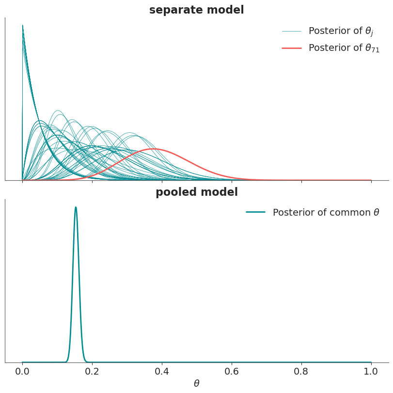

# compute the marginal posterior of alpha and beta in the hierarchical model in a grid
A = np.linspace(0.5, 6, 100)
B = np.linspace(3, 33, 100)
# calculated in logarithms for numerical accuracy
lp = (
  - 5/2 * np.log(A + B[:,None])
  + np.sum(
        gammaln(A + B[:,None])
      - gammaln(A)
      - gammaln(B[:,None])
      + gammaln(A + y[:,None,None])
      + gammaln(B[:,None] + (n - y)[:,None,None])
      - gammaln(A + B[:,None] + n[:,None,None]),
        axis=0
    )
)
# subtract the maximum value to avoid over/underflow in exponentation
lp -= lp.max()
p = np.exp(lp)

# plot the marginal posterior
_, ax = plt.subplots()
ax.imshow(
    p,
    origin='lower',
    aspect='auto',
    extent=(A[0], A[-1], B[0], B[-1])
)
ax.set(xlabel=r'$\alpha$', ylabel=r'$\beta$', title='The marginal posterior of alpha and beta in hierarchical model')
ax.grid(False)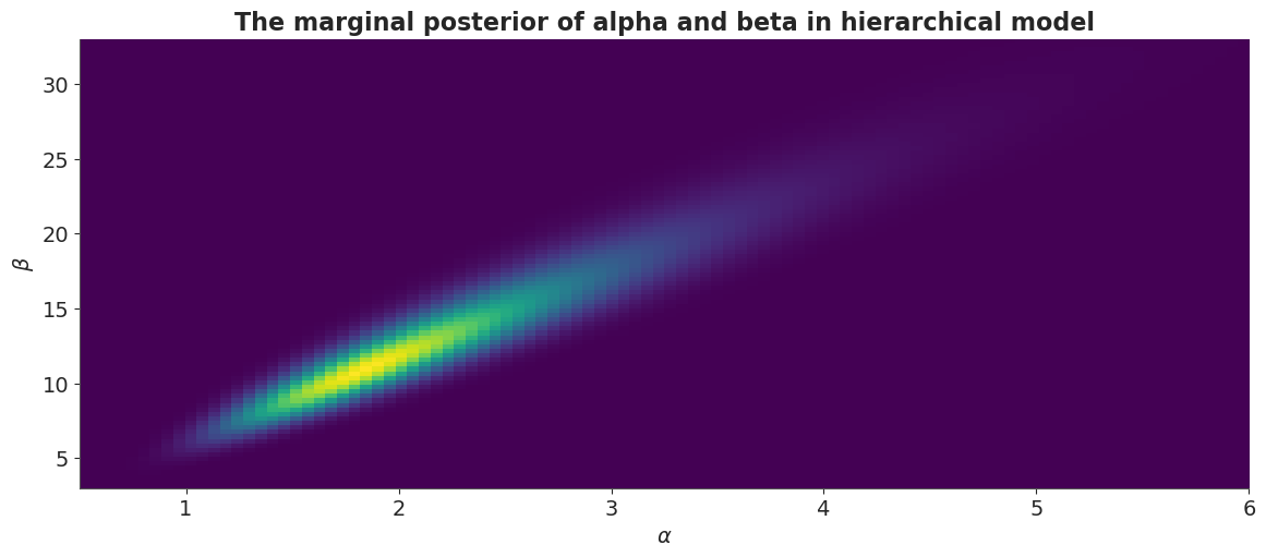

# sample from the posterior grid of alpha and beta
nsamp = 1000
samp_indices = np.unravel_index(
    np.random.choice(p.size, size=nsamp, p=p.ravel()/p.sum()),
    p.shape
)
samp_A = A[samp_indices[1]]
samp_B = B[samp_indices[0]]
# add random jitter, see BDA3 p. 76
samp_A += (np.random.rand(nsamp) - 0.5) * (A[1]-A[0])
samp_B += (np.random.rand(nsamp) - 0.5) * (B[1]-B[0])

fig, (ax_samples, ax_pred) = plt.subplots(2, 1, sharex=True, figsize=(8, 8))

# Posterior samples from Beta(alpha, beta)
ax_samples.plot(
    x,
    beta.pdf(x[:, None], samp_A[:20], samp_B[:20]),
    lw=0.5, color="C0"
)
ax_samples.set(yticks=[], ylim=0,
               title=r'Posterior samples from the distribution of distributions Beta($\alpha$,$\beta$)')

# Predictive distribution for a new theta
mean_pdf = pz.Beta(samp_A[:, None], samp_B[:, None]).pdf(x).mean(axis=0)
ax_pred.plot(x, mean_pdf)
ax_pred.set(yticks=[], ylim=0,
            xlabel=r"$\theta$",
            title=r'Predictive distribution for a new $\theta$ and prior for $\theta_j$');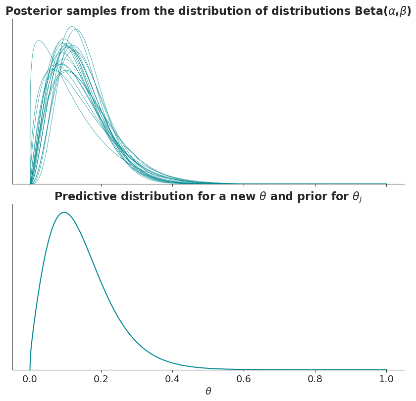

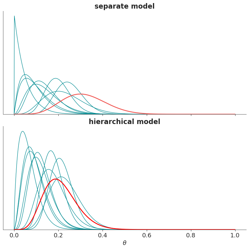
fig, (ax_sep, ax_hier) = plt.subplots(2, 1, sharex=True, figsize=(8, 8))
x = np.linspace(0, 1, 1000)

# Separate model (plot every 7th distribution)
lines = ax_sep.plot(
    x,
    pz.Beta(y[7:-1:7] + 1, n[7:-1:7] - y[7:-1:7] + 1).pdf(x[:, None]),
    color="C0", lw=1
)
lines[-1].set(lw=2, color="C2")
ax_sep.set(yticks=[], ylim=0, title="separate model")

# Hierarchical model (plot every 7th distribution) ---
lines = ax_hier.plot(
    x,
    np.mean(pz.Beta(
            y[7::7] + samp_A[:,None,None],
            n[7::7] - y[7::7] + samp_B[:,None,None]
            ).pdf(x[:,None]), axis=0),
    color='C0', lw=1,
)
lines[-1].set(lw=2, color="r")
ax_hier.set(yticks=[], ylim=0, xlabel=r"$\theta$", title="hierarchical model");