# Elections economy: prior, likelihood, posterior
Source: `ElectionsEconomy/bayes.Rmd`
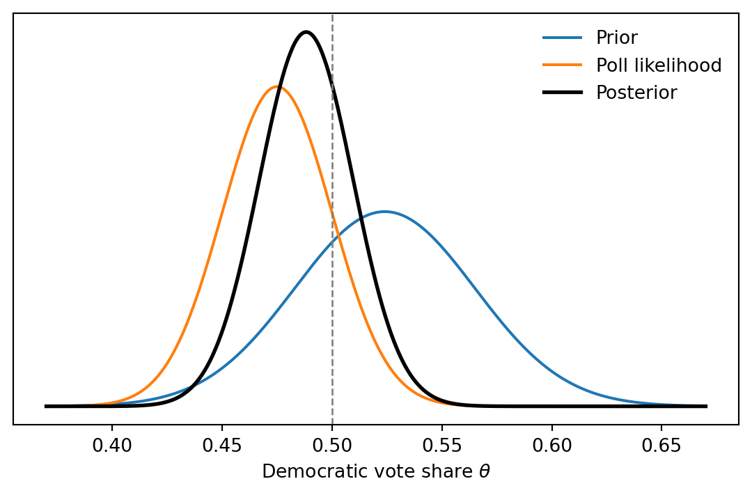
This page is a compact Bayesian information-aggregation example. A previous election/economy model supplies a normal prior for the Democratic vote share, and a new poll supplies an approximately normal likelihood.
## Inputs
```{python}
import numpy as np
import pandas as pd
import matplotlib.pyplot as plt
from scipy.stats import norm, binom

# Prior from a previously fitted model using economic and political conditions.
theta_hat_prior = 0.524
se_prior = 0.041

# Poll: 190 Democratic supporters out of 400 respondents.
n = 400
y = 190
```
## Poll estimate
```{python}
theta_hat_data = y / n
se_data = np.sqrt(theta_hat_data * (1 - theta_hat_data) / n)

pd.Series({
    "prior_mean": theta_hat_prior,
    "prior_se": se_prior,
    "poll_mean": theta_hat_data,
    "poll_se": se_data,
})
```
## Normal-normal posterior calculation
With a normal prior and normal approximation to the poll likelihood, the posterior precision is the sum of prior and data precisions.
```{python}
prior_precision = 1 / se_prior**2
data_precision = 1 / se_data**2

theta_hat_bayes = (
    theta_hat_prior * prior_precision + theta_hat_data * data_precision
) / (prior_precision + data_precision)
se_bayes = np.sqrt(1 / (prior_precision + data_precision))

pd.Series({
    "posterior_mean": theta_hat_bayes,
    "posterior_se": se_bayes,
    "posterior_pr_dem_above_50": 1 - norm.cdf(0.5, theta_hat_bayes, se_bayes),
})
```
The posterior mean falls between the prior estimate and the raw poll estimate, closer to whichever source has smaller standard error.
## Plot prior, likelihood, and posterior
```{python}
grid = np.linspace(0.37, 0.67, 1000)
prior_pdf = norm.pdf(grid, theta_hat_prior, se_prior)
lik_pdf = norm.pdf(grid, theta_hat_data, se_data)
post_pdf = norm.pdf(grid, theta_hat_bayes, se_bayes)

fig, ax = plt.subplots(figsize=(7, 4))
ax.plot(grid, prior_pdf, label="Prior")
ax.plot(grid, lik_pdf, label="Poll likelihood")
ax.plot(grid, post_pdf, label="Posterior", color="black", linewidth=2)
ax.axvline(0.5, color="gray", linestyle="--", linewidth=1)
ax.set_xlabel(r"Democratic vote share $\theta$")
ax.set_yticks([])
ax.legend(frameon=False)
```
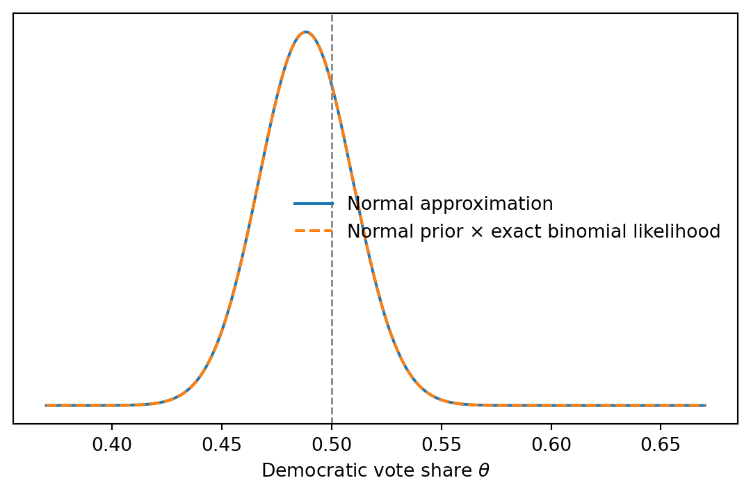
## Exact-binomial comparison
The R original uses the normal approximation. For this sample size it is also useful to compare with the exact binomial likelihood on a grid. We keep the same normal prior and normalize numerically.
```{python}
prior = norm.pdf(grid, theta_hat_prior, se_prior)
lik_binom = binom.pmf(y, n, grid)
post_grid = prior * lik_binom
post_grid = post_grid / np.trapezoid(post_grid, grid)

post_grid_mean = np.trapezoid(grid * post_grid, grid)
post_grid_sd = np.sqrt(np.trapezoid((grid - post_grid_mean) ** 2 * post_grid, grid))

pd.Series({
    "normal_posterior_mean": theta_hat_bayes,
    "normal_posterior_sd": se_bayes,
    "grid_binomial_posterior_mean": post_grid_mean,
    "grid_binomial_posterior_sd": post_grid_sd,
})
```
```{python}
fig, ax = plt.subplots(figsize=(7, 4))
ax.plot(grid, post_pdf, label="Normal approximation")
ax.plot(grid, post_grid, linestyle="--", label="Normal prior × exact binomial likelihood")
ax.axvline(0.5, color="gray", linestyle="--", linewidth=1)
ax.set_xlabel(r"Democratic vote share $\theta$")
ax.set_yticks([])
ax.legend(frameon=False)
```
## CmdStanPy version
This is overkill for a one-parameter conjugate calculation, but it is the direct Stan version of the same model.
```{python}
#| eval: false
from pathlib import Path
from cmdstanpy import CmdStanModel

stan_code = """
data {
  int<lower=0> n;
  int<lower=0, upper=n> y;
  real prior_mean;
  real<lower=0> prior_sd;
}
parameters {
  real<lower=0, upper=1> theta;
}
model {
  theta ~ normal(prior_mean, prior_sd);
  y ~ binomial(n, theta);
}
generated quantities {
  int y_rep = binomial_rng(n, theta);
}
"""
Path("elections_bayes.stan").write_text(stan_code)
model = CmdStanModel(stan_file="elections_bayes.stan")
fit = model.sample(
    data={"n": n, "y": y, "prior_mean": theta_hat_prior, "prior_sd": se_prior},
    chains=4,
    seed=123,
)
fit.summary().loc[["theta"]]
```