# Elections Economy: uncertainty in the regression line
Source: `ElectionsEconomy/hills.Rmd`
This page visualizes uncertainty in the intercept and slope of the Hibbs election-economy regression. The R version combines least squares summaries with posterior draws from `stan_glm` under a flat prior. In this Python port, `statsmodels` gives the least-squares fit and we draw from the large-sample Gaussian approximation to the joint distribution of the coefficients.
## Setup and data
```{python}
from pathlib import Path
import numpy as np
import pandas as pd
import matplotlib.pyplot as plt
import statsmodels.formula.api as smf
from scipy.stats import multivariate_normal

root = Path("../../ROS-Examples")
hibbs = pd.read_csv(root / "ElectionsEconomy/data/hibbs.dat", sep=r"\s+")
rng = np.random.default_rng(7007)
hibbs.head()
```
## Least squares fit
```{python}
model = smf.ols("vote ~ growth", data=hibbs).fit()
model.summary()
```
```{python}
coef = model.params[["Intercept", "growth"]].to_numpy()
cov = model.cov_params().loc[["Intercept", "growth"], ["Intercept", "growth"]].to_numpy()
se = model.bse[["Intercept", "growth"]].to_numpy()
pd.DataFrame({"estimate": coef, "std_err": se}, index=["a", "b"])
```
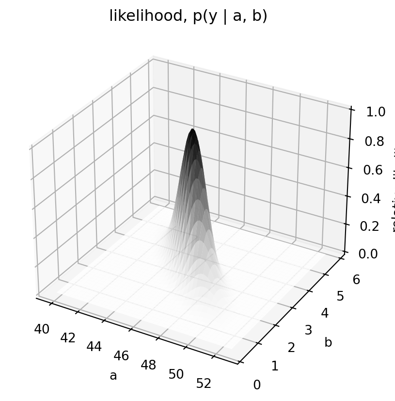
## Likelihood for intercept and slope
For a Gaussian regression with residual variance fixed at its estimate, the likelihood for `(a, b)` is proportional to a bivariate normal density centered at the least-squares estimate.
```{python}
a_grid = np.linspace(coef[0] - 4 * se[0], coef[0] + 4 * se[0], 80)
b_grid = np.linspace(coef[1] - 4 * se[1], coef[1] + 4 * se[1], 80)
A, B = np.meshgrid(a_grid, b_grid, indexing="ij")
pos = np.dstack([A, B])
Z = multivariate_normal(mean=coef, cov=cov).pdf(pos)
Z = Z / Z.max()

fig = plt.figure(figsize=(7, 5))
ax = fig.add_subplot(111, projection="3d")
ax.plot_surface(A, B, Z, cmap="Greys", linewidth=0, alpha=0.85)
ax.set_xlabel("a")
ax.set_ylabel("b")
ax.set_zlabel("relative likelihood")
ax.set_title("likelihood, p(y | a, b)")
```
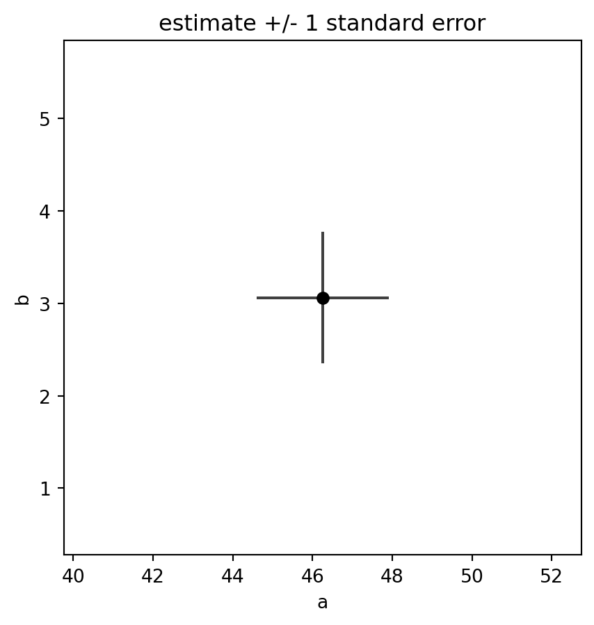
## Estimate plus one-standard-error cross
```{python}
fig, ax = plt.subplots(figsize=(5, 5))
ax.set_xlim(a_grid.min(), a_grid.max())
ax.set_ylim(b_grid.min(), b_grid.max())
ax.plot([coef[0], coef[0]], [coef[1] - se[1], coef[1] + se[1]], color="0.25")
ax.plot([coef[0] - se[0], coef[0] + se[0]], [coef[1], coef[1]], color="0.25")
ax.scatter([coef[0]], [coef[1]], color="black", zorder=3)
ax.set_xlabel("a")
ax.set_ylabel("b")
ax.set_title("estimate +/- 1 standard error")
```
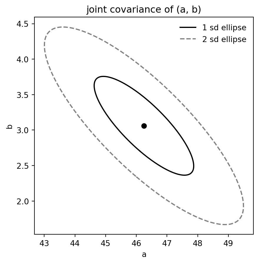
## Joint covariance ellipse
```{python}
def covariance_ellipse(mean, cov, radius=1.0, n=400):
    theta = np.linspace(0, 2 * np.pi, n)
    circle = np.column_stack([np.cos(theta), np.sin(theta)])
    vals, vecs = np.linalg.eigh(cov)
    transform = vecs @ np.diag(np.sqrt(vals))
    return mean + radius * circle @ transform.T

ell_1 = covariance_ellipse(coef, cov, radius=1)
ell_2 = covariance_ellipse(coef, cov, radius=2)

fig, ax = plt.subplots(figsize=(5, 5))
ax.plot(ell_1[:, 0], ell_1[:, 1], color="black", label="1 sd ellipse")
ax.plot(ell_2[:, 0], ell_2[:, 1], color="0.5", linestyle="--", label="2 sd ellipse")
ax.scatter([coef[0]], [coef[1]], color="black")
ax.set_xlabel("a")
ax.set_ylabel("b")
ax.set_title("joint covariance of (a, b)")
ax.legend(frameon=False)
```
The tilted ellipse is the key display: intercept and slope are negatively correlated because the fitted line can pivot through the observed range of `growth`.
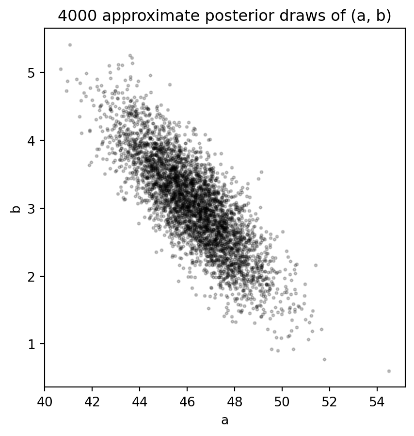
## Approximate posterior draws with a flat prior
```{python}
draws = rng.multivariate_normal(coef, cov, size=4000)
draws_df = pd.DataFrame(draws, columns=["a", "b"])
draws_df.describe(percentiles=[0.05, 0.5, 0.95])
```
```{python}
fig, ax = plt.subplots(figsize=(5, 5))
ax.scatter(draws_df["a"], draws_df["b"], s=4, alpha=0.2, color="black")
ax.set_xlabel("a")
ax.set_ylabel("b")
ax.set_title("4000 approximate posterior draws of (a, b)")
```
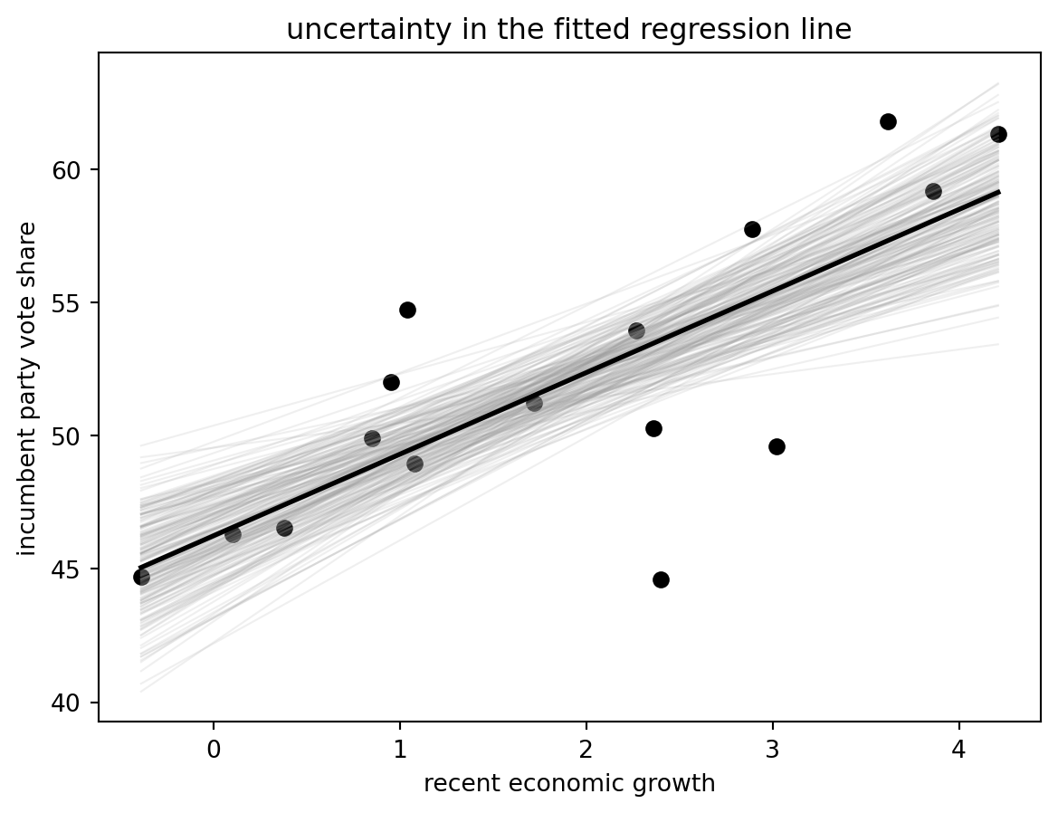
```{python}
x_grid = np.linspace(hibbs["growth"].min(), hibbs["growth"].max(), 100)
line_draws = draws[:200, 0, None] + draws[:200, 1, None] * x_grid

fig, ax = plt.subplots()
ax.scatter(hibbs["growth"], hibbs["vote"], color="black")
for line in line_draws:
    ax.plot(x_grid, line, color="0.6", alpha=0.15, linewidth=0.8)
ax.plot(x_grid, coef[0] + coef[1] * x_grid, color="black", linewidth=2)
ax.set_xlabel("recent economic growth")
ax.set_ylabel("incumbent party vote share")
ax.set_title("uncertainty in the fitted regression line")
```