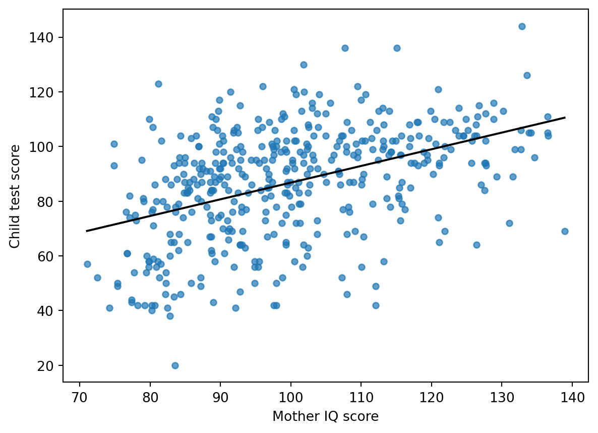
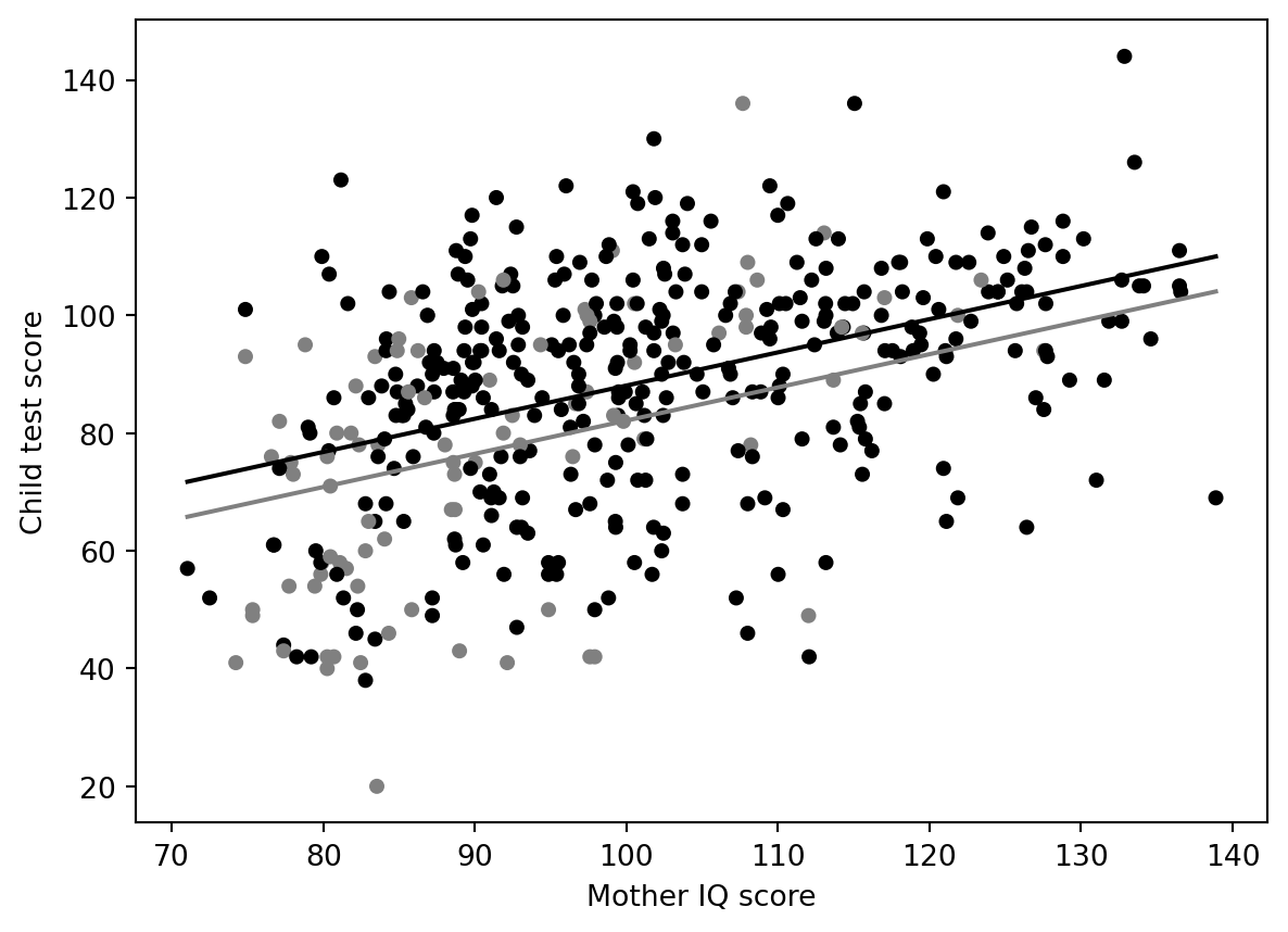
KidIQ: multiple linear regression

Source: KidIQ/kidiq.Rmd

This page ports the core rstanarm::stan_glm examples to Python with the formula-first lapylace interface.

Load data

from pathlib import Path
import pandas as pd
import lapylace as lp
import numpy as np
import matplotlib.pyplot as plt

root = Path("../../ROS-Examples")
kidiq = pd.read_csv(root / "KidIQ/data/kidiq.csv")
kidiq.head()

	kid_score	mom_hs	mom_iq	mom_work	mom_age
0	65	1	121.117529	4	27
1	98	1	89.361882	4	25
2	85	1	115.443165	4	27
3	83	1	99.449639	3	25
4	115	1	92.745710	4	27

def coef_medians(fit):
    return pd.Series(
        [np.median(fit.alpha_draws()), *np.median(fit.beta_draws(), axis=0)],
        index=["Intercept", *fit.columns],
    )

def fit_gaussian(formula, seed):
    return lp.stan_glm(
        formula,
        data=kidiq,
        family=lp.gaussian(),
        prior=lp.normal(0, 10),
        prior_intercept=lp.normal(0, 30),
        prior_aux=lp.exponential(30),
        chains=4,
        parallel_chains=4,
        iter_warmup=500,
        iter_sampling=1000,
        seed=seed,
        refresh=100,
    )

Single binary predictor

R original:

stan_glm(kid_score ~ mom_hs, data=kidiq)

Python:

fit_1 = fit_gaussian("kid_score ~ mom_hs", seed=16101)
fit_1.summary(["alpha", "beta", "sigma"])

	Mean	MCSE	StdDev	5%	50%	95%	N_Eff	N_Eff/s	R_hat
alpha	77.6974	0.052610	2.050450	74.30130	77.7053	81.0702	1519.000000	1718.320000	1.000130
beta[1]	11.4633	0.059545	2.304050	7.68109	11.4425	15.3118	1497.260000	1693.740000	0.999596
sigma	19.8946	0.015305	0.679249	18.78570	19.8853	21.0376	1969.607443	2228.062719	1.000275

Single continuous predictor

fit_2 = fit_gaussian("kid_score ~ mom_iq", seed=16102)
coef_2 = coef_medians(fit_2)
coef_2.round(2)

Intercept    24.77
mom_iq        0.62
dtype: float64

ax = kidiq.plot.scatter("mom_iq", "kid_score", alpha=0.7)
xs = np.linspace(kidiq.mom_iq.min(), kidiq.mom_iq.max(), 100)
ax.plot(xs, coef_2["Intercept"] + coef_2["mom_iq"] * xs, color="black")
ax.set_xlabel("Mother IQ score")
ax.set_ylabel("Child test score")

Text(0, 0.5, 'Child test score')

Two predictors

fit_3 = fit_gaussian("kid_score ~ mom_hs + mom_iq", seed=16103)
coef_3 = coef_medians(fit_3)
coef_3.round(2)

Intercept    24.65
mom_hs        5.64
mom_iq        0.58
dtype: float64

Two fitted lines, no interaction:

fig, ax = plt.subplots()
colors = np.where(kidiq.mom_hs == 1, "black", "gray")
ax.scatter(kidiq.mom_iq, kidiq.kid_score, c=colors, s=18)
for hs, color in [(0, "gray"), (1, "black")]:
    ax.plot(xs, coef_3["Intercept"] + coef_3["mom_hs"]*hs + coef_3["mom_iq"]*xs, color=color)
ax.set_xlabel("Mother IQ score")
ax.set_ylabel("Child test score")

Text(0, 0.5, 'Child test score')

Interaction model

fit_4 = fit_gaussian("kid_score ~ mom_hs * mom_iq", seed=16104)
coef_medians(fit_4).round(2)

Intercept        16.29
mom_hs           15.96
mom_iq            0.67
mom_hs:mom_iq    -0.12
dtype: float64

Stan model generated by Lapylace

lapylace generates the same Gaussian regression structure behind the formula call.

data {
  int<lower=1> N;
  int<lower=1> K;
  matrix[N, K] X;
  vector[N] y;
}
parameters {
  vector[K] beta;
  real<lower=0> sigma;
}
model {
  beta ~ normal(0, 10);
  sigma ~ exponential(1);
  y ~ normal(X * beta, sigma);
}

BlackJAX relevance

This example is a good teaching case for writing the Gaussian regression log density by hand, but lapylace is preferable for the main exposition. BlackJAX becomes useful when we want explicit NUTS mechanics or JAX-vectorized repeated simulations.