# Mesquite yields: transformations and predictive comparison
Source: `Mesquite/mesquite.Rmd`
The mesquite example compares a model for raw bush weight to log-log models. The original uses Bayesian GLMs with LOO/K-fold; this Python port uses OLS analogues and cross-validated predictive error to show the same modeling issue.
```{python}
from pathlib import Path
import numpy as np
import pandas as pd
import matplotlib.pyplot as plt
import statsmodels.formula.api as smf
from sklearn.model_selection import KFold, cross_val_score
from sklearn.compose import ColumnTransformer
from sklearn.preprocessing import OneHotEncoder, StandardScaler
from sklearn.pipeline import make_pipeline
from sklearn.linear_model import LinearRegression

root = Path("../../ROS-Examples")
mesquite = pd.read_table(root / "Mesquite/data/mesquite.dat", sep=r"\s+")
mesquite.head()
```
## Raw-scale regression
```{python}
fit1 = smf.ols("weight ~ diam1 + diam2 + canopy_height + total_height + density + C(group)", data=mesquite).fit()
fit1.summary()
```
## Log-log regression
```{python}
mesquite = mesquite.assign(
    log_weight=np.log(mesquite.weight),
    log_diam1=np.log(mesquite.diam1),
    log_diam2=np.log(mesquite.diam2),
    log_canopy_height=np.log(mesquite.canopy_height),
    log_total_height=np.log(mesquite.total_height),
    log_density=np.log(mesquite.density),
)
fit2 = smf.ols("log_weight ~ log_diam1 + log_diam2 + log_canopy_height + log_total_height + log_density + C(group)", data=mesquite).fit()
fit2.summary()
```
## K-fold predictive comparison
```{python}
cv = KFold(n_splits=10, shuffle=True, random_state=4587)
raw_X = mesquite[["diam1", "diam2", "canopy_height", "total_height", "density", "group"]]
log_X = mesquite[["log_diam1", "log_diam2", "log_canopy_height", "log_total_height", "log_density", "group"]]
pre_raw = ColumnTransformer([("num", StandardScaler(), ["diam1", "diam2", "canopy_height", "total_height", "density"]), ("grp", OneHotEncoder(drop="first"), ["group"])])
pre_log = ColumnTransformer([("num", StandardScaler(), ["log_diam1", "log_diam2", "log_canopy_height", "log_total_height", "log_density"]), ("grp", OneHotEncoder(drop="first"), ["group"])])
raw_pipe = make_pipeline(pre_raw, LinearRegression())
log_pipe = make_pipeline(pre_log, LinearRegression())
raw_rmse = -cross_val_score(raw_pipe, raw_X, mesquite.weight, cv=cv, scoring="neg_root_mean_squared_error")
log_rmse = -cross_val_score(log_pipe, log_X, mesquite.log_weight, cv=cv, scoring="neg_root_mean_squared_error")
print(raw_rmse.mean(), log_rmse.mean())
```
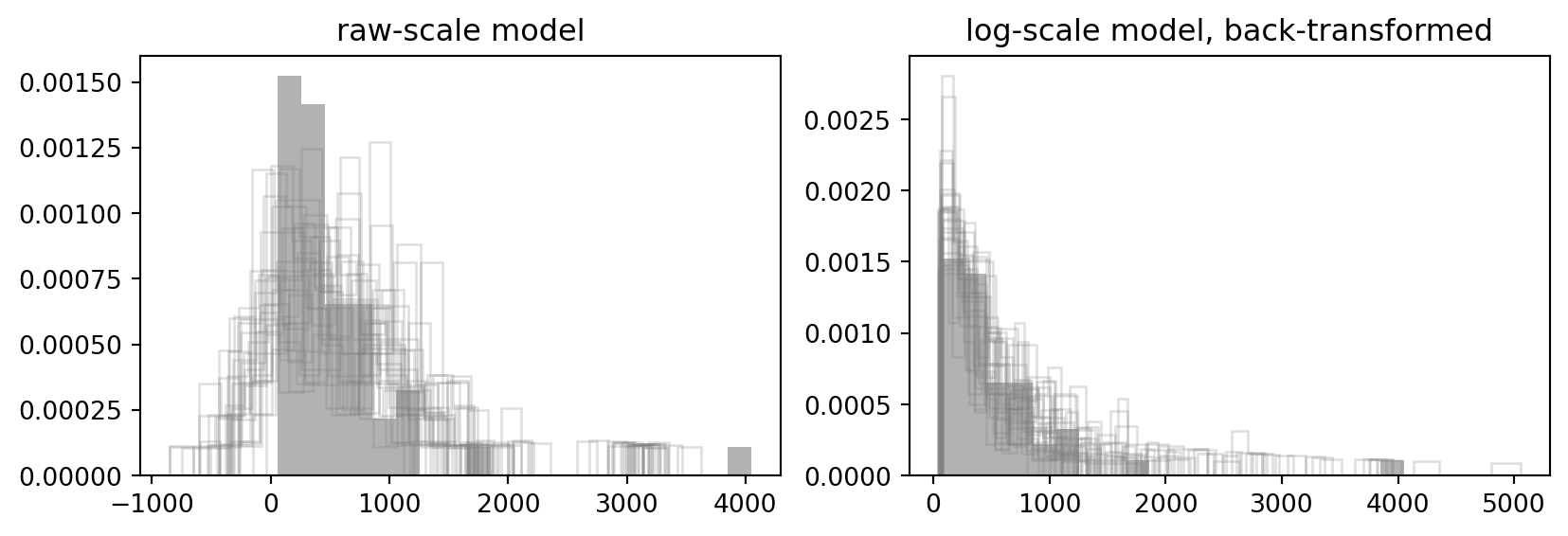
## Posterior-predictive-check analogue
```{python}
rng = np.random.default_rng(4587)
yhat1 = fit1.fittedvalues.to_numpy()
yhat2 = np.exp(fit2.fittedvalues.to_numpy())
sigma1 = np.sqrt(fit1.mse_resid)
sigma2 = np.sqrt(fit2.mse_resid)
yrep1 = rng.normal(yhat1, sigma1, size=(100, len(yhat1)))
yrep2 = np.exp(rng.normal(fit2.fittedvalues.to_numpy(), sigma2, size=(100, len(yhat2))))
fig, axs = plt.subplots(1, 2, figsize=(10, 3))
axs[0].hist(mesquite.weight, bins=20, density=True, color="black", alpha=.3)
for row in yrep1[:25]: axs[0].hist(row, bins=20, density=True, histtype="step", color="gray", alpha=.25)
axs[0].set_title("raw-scale model")
axs[1].hist(mesquite.weight, bins=20, density=True, color="black", alpha=.3)
for row in yrep2[:25]: axs[1].hist(row, bins=20, density=True, histtype="step", color="gray", alpha=.25)
axs[1].set_title("log-scale model, back-transformed")
```
## Canopy volume simplification
```{python}
mesquite["canopy_volume"] = mesquite.diam1 * mesquite.diam2 * mesquite.canopy_height
fit3 = smf.ols("log_weight ~ np.log(canopy_volume)", data=mesquite).fit()
pd.DataFrame({"model": ["full log model", "canopy volume"], "aic": [fit2.aic, fit3.aic], "r2": [fit2.rsquared, fit3.rsquared]})
```