Heights and weights: normals, mixtures, and lognormals

Source: CentralLimitTheorem/heightweight.Rmd

This example uses summary histogram counts to show where normal approximations work and where mixtures or transformations are better.

Code

import numpy as np
import matplotlib.pyplot as plt
from scipy.stats import norm, lognorm

Summary counts

Code

height_counts_women = np.array([80,107,296,695,1612,2680,4645,8201,9948,11733,10270,9942,6181,3990,2131,1154,245,257,0,0,0,0]) * 10339/74167
weight_counts_women = np.array([362,1677,4572,9363,11420,12328,9435,7023,5047,3621,2753,2081,1232,887,2366]) * 10339/74167
height_counts_men = np.array([0,0,0,0,0,0,0,542,668,1221,2175,4213,5535,7980,9566,9578,8867,6716,5019,2745,1464,1263]) * 9983/67552
height_counts = height_counts_women + height_counts_men
heights = np.arange(54, 76)

Histograms from aggregated data

Code

fig, axs = plt.subplots(1, 3, figsize=(11, 3))
axs[0].bar(heights, height_counts_women, width=0.9)
axs[0].set_title("women's heights")
axs[1].bar(heights, height_counts, width=0.9)
axs[1].set_title("all adult heights")
axs[2].bar(np.arange(len(weight_counts_women)), weight_counts_women, width=0.9)
axs[2].set_title("women's weights")
for ax in axs: ax.set_ylabel("count")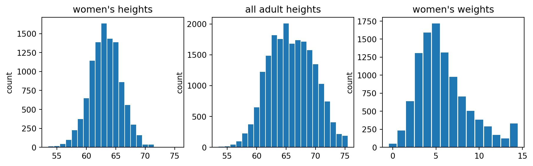

Normal and mixture approximations

Code

x = np.linspace(52, 81, 500)
fig, axs = plt.subplots(1, 3, figsize=(11, 3))
axs[0].plot(x, norm.pdf(x, 63.7, 2.7))
axs[0].set_title("women: approximately normal")
axs[1].plot(x, norm.pdf(x, 69.1, 2.9))
axs[1].set_title("men: approximately normal")
axs[2].plot(x, 0.52*norm.pdf(x, 63.7, 2.7) + 0.48*norm.pdf(x, 69.1, 2.9))
axs[2].set_title("all adults: mixture, not normal")
for ax in axs: ax.set_xlabel("height (inches)")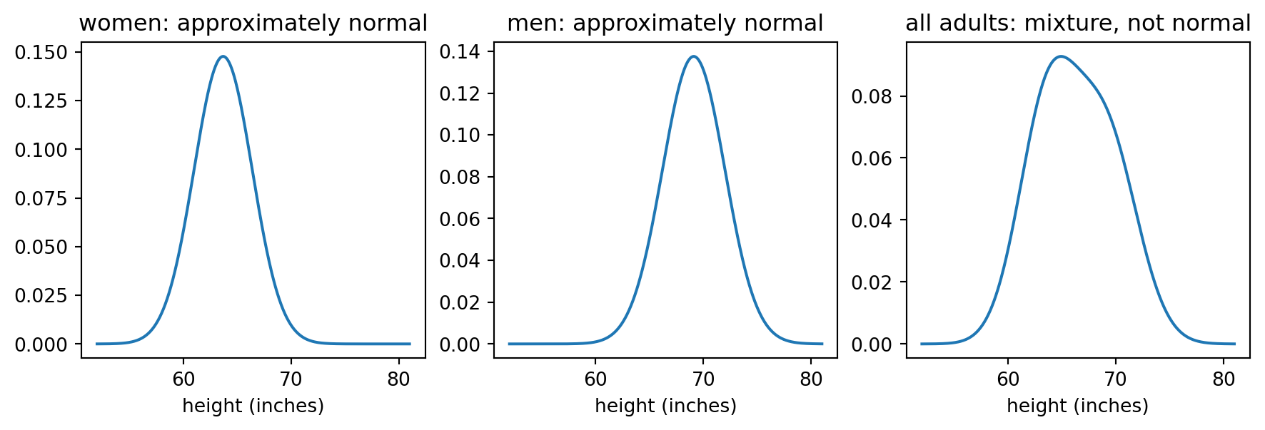

Log weights

Code

x_log = np.linspace(4, 6, 500)
x_w = np.linspace(50, 350, 500)
fig, axs = plt.subplots(1, 2, figsize=(8, 3))
axs[0].plot(x_log, norm.pdf(x_log, 5.13, 0.17))
axs[0].set_title("log weights of men")
axs[1].plot(x_w, lognorm.pdf(x_w, s=0.17, scale=np.exp(5.13)))
axs[1].set_title("weights of men: lognormal")

Text(0.5, 1.0, 'weights of men: lognormal')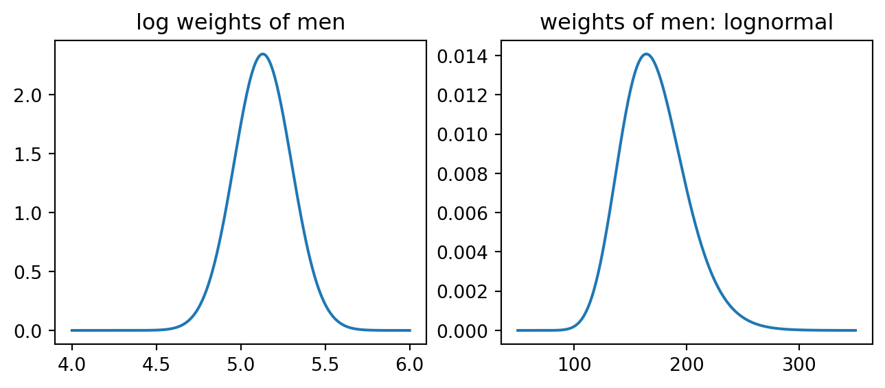

The statistical point is that marginal human heights are close to normal within sex, but the pooled adult distribution is visibly a mixture. Weights are often better approximated after a logarithmic transformation.