from pathlib import Path
import numpy as np
import pandas as pd
import matplotlib.pyplot as plt
import lapylace as lp

root = Path("../../ROS-Examples")

def coef_medians(fit):
    return pd.Series(
        [np.median(fit.alpha_draws()), *np.median(fit.beta_draws(), axis=0)],
        index=["Intercept", *fit.columns],
    )

def fit_glm(formula, data, family=None, seed=1, prior_scale=2.5, intercept_scale=5, aux_scale=10, **kwargs):
    return lp.stan_glm(
        formula,
        data=data,
        family=family or lp.gaussian(),
        prior=lp.normal(0, prior_scale),
        prior_intercept=lp.normal(0, intercept_scale),
        prior_aux=lp.exponential(aux_scale),
        chains=2,
        parallel_chains=2,
        iter_warmup=300,
        iter_sampling=500,
        seed=seed,
        refresh=100,
        **kwargs,
)Poisson regression simulation
Source: PoissonExample/poisson_regression.Rmd
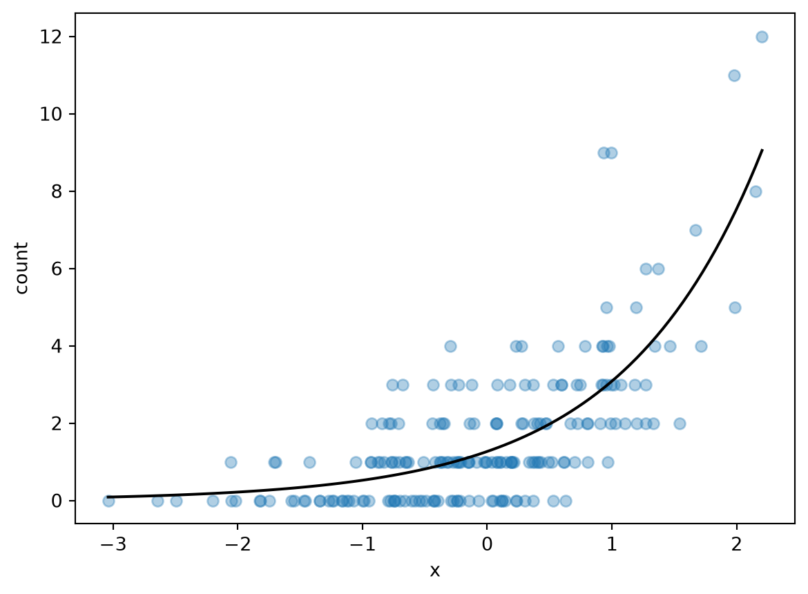
This page simulates log-linear count data and fits the corresponding Poisson model with lapylace.
Simulation
rng = np.random.default_rng(18301)
n = 200
fake = pd.DataFrame({"x": rng.normal(size=n)})
fake["lambda"] = np.exp(0.4 + 0.8 * fake["x"])
fake["y"] = rng.poisson(fake["lambda"])
fake.head()| x | lambda | y | |
|---|---|---|---|
| 0 | -0.144804 | 1.328641 | 0 |
| 1 | 1.017549 | 3.367058 | 3 |
| 2 | -1.425941 | 0.476755 | 1 |
| 3 | -0.070408 | 1.410118 | 0 |
| 4 | 1.181508 | 3.838980 | 3 |
fit = fit_glm("y ~ x", fake, family=lp.poisson(), seed=18302, prior_scale=2.5, intercept_scale=5)
fit.summary(["alpha", "beta"]) | Mean | MCSE | StdDev | 5% | 50% | 95% | N_Eff | N_Eff/s | R_hat | |
|---|---|---|---|---|---|---|---|---|---|
| alpha | 0.233930 | 0.002917 | 0.066142 | 0.116435 | 0.235343 | 0.343038 | 514.114 | 7140.47 | 1.002020 |
| beta[1] | 0.890479 | 0.003023 | 0.062939 | 0.785463 | 0.890828 | 0.990079 | 433.446 | 6020.09 | 0.998592 |
grid = pd.DataFrame({"x": np.linspace(fake.x.min(), fake.x.max(), 100)})
pred = fit.posterior_epred(grid)
fig, ax = plt.subplots()
ax.scatter(fake.x, fake.y, alpha=.35)
ax.plot(grid.x, pred.mean(axis=0), color="black")
ax.set_xlabel("x")
ax.set_ylabel("count")
Text(0, 0.5, 'count')