Chapter 10, demo 2

Bayesian data analysis

Importance sampling example

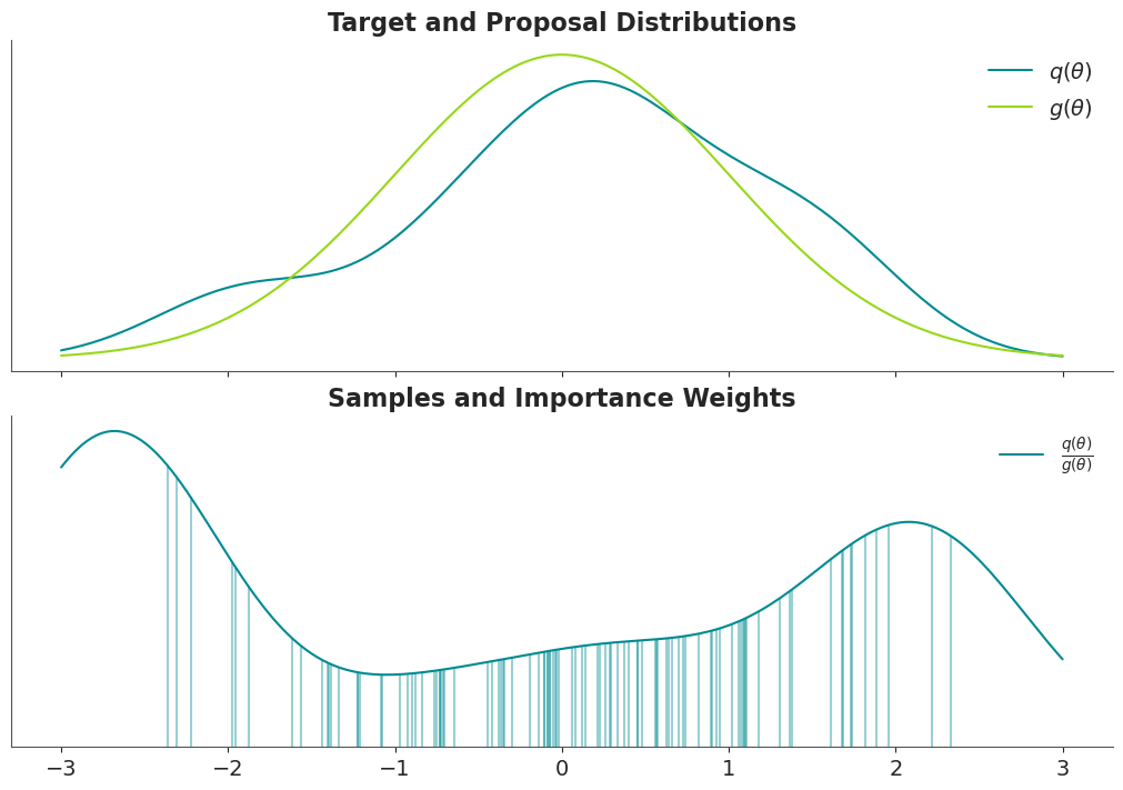
In importance sampling the proposal \(g(\theta)\) does not need to form an envelope over the target \(q(\theta)\). When computing the expectations, draws are weighted based on the ratio of the proposal and the target.

\[ \mathrm{E}[f(\theta)] \approx \frac{\sum_s w_s f(\theta^{(s)})}{\sum_s w_s}, \qquad \text{where} \quad w_s = \frac{q(\theta^{(s)})}{g(\theta^{(s)})} \qquad. \]

import numpy as np
from scipy.stats import gaussian_kde
import preliz as pz

import matplotlib.pyplot as plt
pz.style.use('preliz-doc')

# fake interesting distribution
x = np.linspace(-3, 3, 200)
r = np.array([ 1.1 ,  1.3 , -0.1 , -0.7 ,  0.2 , -0.4 ,  0.06, -1.7 ,
               1.7 ,  0.3 ,  0.7 ,  1.6 , -2.06, -0.74,  0.2 ,  0.5 ])
# Estimate the density (named q, to emphasize that it does not need to be
# normalized). Parameter bw_method=0.48 is used to mimic the outcome of the
# kernelp function in Matlab.
q_func = gaussian_kde(r, bw_method=0.48)
q = q_func.evaluate(x)

# importance sampling example
dist = pz.Normal(0, 1)
g = dist.pdf(x)
w = q / g
r = np.random.randn(100)
r = r[np.abs(r) < 3] # remove samples out of the grid
wr = q_func.evaluate(r)/dist.pdf(r)

_, (ax1, ax2) = plt.subplots(2, 1, figsize=(10, 7), sharex=True)

# Top plot: target and proposal
ax1.plot(x, q, label=r'$q(\theta)$')
ax1.plot(x, g, label=r'$g(\theta)$')
ax1.set(yticks=[], title='Target and Proposal Distributions')
ax1.legend()

# Bottom plot: importance weights
ax2.plot(x, w, label=r'$\frac{q(\theta)}{g(\theta)}$')
ax2.vlines(r, 0, wr, color='C0', alpha=0.4)
ax2.set(ylim=0, yticks=[], title='Samples and Importance Weights')
ax2.legend();