Code
import numpy as np
import pandas as pd
import matplotlib.pyplot as plt
from scipy.special import expit
import statsmodels.formula.api as smf

rng = np.random.default_rng(20260531)Source: FakeMidtermFinal/simulation_based_design.Rmd
This example simulates randomized and biased treatment assignments for student grades. The estimand is a treatment effect of 5 points. Randomization protects the simple difference in means; a useful pre-test reduces uncertainty; biased assignment creates confounding that adjustment can partly repair.
import numpy as np
import pandas as pd
import matplotlib.pyplot as plt
from scipy.special import expit
import statsmodels.formula.api as smf
rng = np.random.default_rng(20260531)n = 100
y_if_control = rng.normal(60, 20, size=n)
y_if_treated = y_if_control + 5
z = rng.permutation(np.repeat([0, 1], n // 2))
y = np.where(z == 1, y_if_treated, y_if_control)
fake = pd.DataFrame({"y": y, "z": z})
diff = fake.loc[fake.z == 1, "y"].mean() - fake.loc[fake.z == 0, "y"].mean()
se_diff = np.sqrt(
fake.loc[fake.z == 0, "y"].var(ddof=1) / (z == 0).sum()
+ fake.loc[fake.z == 1, "y"].var(ddof=1) / (z == 1).sum()
)
pd.Series({"difference in means": diff, "standard error": se_diff}).round(2)difference in means -0.85
standard error 3.57
dtype: float64fit_1a = smf.ols("y ~ z", data=fake).fit()
fake["x"] = rng.normal(50, 20, size=n)
fit_1b = smf.ols("y ~ z + x", data=fake).fit()
pd.DataFrame({
"simple": [fit_1a.params["z"], fit_1a.bse["z"]],
"adjusted for irrelevant x": [fit_1b.params["z"], fit_1b.bse["z"]],
}, index=["estimate", "std_error"]).round(2)| simple | adjusted for irrelevant x | |
|---|---|---|
| estimate | -0.85 | -0.60 |
| std_error | 3.57 | 3.59 |
An unrelated covariate does not systematically improve the treatment-effect estimate.
true_ability = rng.normal(50, 16, size=n)
x = true_ability + rng.normal(0, 12, size=n)
y_if_control = true_ability + rng.normal(0, 12, size=n) + 10
y_if_treated = y_if_control + 5
z = rng.permutation(np.repeat([0, 1], n // 2))
y = np.where(z == 1, y_if_treated, y_if_control)
fake_2 = pd.DataFrame({"x": x, "y": y, "z": z})

fit_2a = smf.ols("y ~ z", data=fake_2).fit()
fit_2b = smf.ols("y ~ z + x", data=fake_2).fit()

pd.DataFrame({
    "simple": [fit_2a.params["z"], fit_2a.bse["z"]],
    "adjusted for pre-test": [fit_2b.params["z"], fit_2b.bse["z"]],
}, index=["estimate", "std_error"]).round(2)| simple | adjusted for pre-test | |
|---|---|---|
| estimate | -0.13 | 0.12 |
| std_error | 3.78 | 3.15 |
Because the pre-test is predictive of the outcome, adjustment typically reduces the standard error in a randomized experiment.
Now treatment is more likely for students with lower pre-test scores:
z_biased = rng.binomial(1, expit(-(x - 50) / 20))
y_biased = np.where(z_biased == 1, y_if_treated, y_if_control)
fake_3 = pd.DataFrame({"x": x, "y": y_biased, "z": z_biased})xx = np.linspace(0, 100, 200)
fig, ax = plt.subplots(figsize=(6, 3.5))
ax.scatter(x, np.where(z_biased == 1, 0.99, 0.01), s=22, alpha=0.7)
ax.plot(xx, expit(-(xx - 50) / 20), color="black")
ax.set_ylim(0, 1)
ax.set_xlabel("Pre-test score")
ax.set_ylabel("Pr(z=1)")
ax.set_title("Biased assignment: lower pre-test scores are treated more often")Text(0.5, 1.0, 'Biased assignment: lower pre-test scores are treated more often')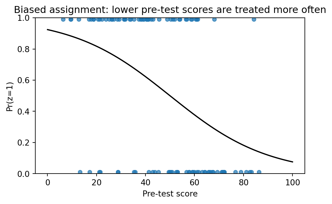
fit_3a = smf.ols("y ~ z", data=fake_3).fit()
fit_3b = smf.ols("y ~ z + x", data=fake_3).fit()

pd.DataFrame({
    "simple": [fit_3a.params["z"], fit_3a.bse["z"]],
    "adjusted for pre-test": [fit_3b.params["z"], fit_3b.bse["z"]],
}, index=["estimate", "std_error"]).round(2)| simple | adjusted for pre-test | |
|---|---|---|
| estimate | -7.20 | 2.31 |
| std_error | 3.61 | 3.63 |
def experiment(rng, n=100):
    true_ability = rng.normal(50, 16, size=n)
    x = true_ability + rng.normal(0, 12, size=n)
    y_if_control = true_ability + rng.normal(0, 12, size=n) + 10
    y_if_treated = y_if_control + 5
    z = rng.binomial(1, expit(-(x - 50) / 20))
    y = np.where(z == 1, y_if_treated, y_if_control)
    dat = pd.DataFrame({"x": x, "y": y, "z": z})
    simple = smf.ols("y ~ z", data=dat).fit()
    adjusted = smf.ols("y ~ z + x", data=dat).fit()
    return pd.DataFrame({
        "model": ["simple", "adjusted"],
        "estimate": [simple.params["z"], adjusted.params["z"]],
        "std_error": [simple.bse["z"], adjusted.bse["z"]],
    })

results = pd.concat([experiment(rng, n) for _ in range(50)], keys=range(50), names=["rep"])
results.groupby("model")[["estimate", "std_error"]].mean().round(2)| estimate | std_error | |
|---|---|---|
| model | ||
| adjusted | 5.33 | 3.39 |
| simple | -5.67 | 3.87 |
fig, ax = plt.subplots(figsize=(6, 3.5))
for model, group in results.reset_index().groupby("model"):
    ax.hist(group["estimate"], bins=12, alpha=0.6, label=model)
ax.axvline(5, color="black", linestyle="--", label="true effect")
ax.set_xlabel("estimated treatment effect")
ax.set_ylabel("replications")
ax.legend(frameon=False)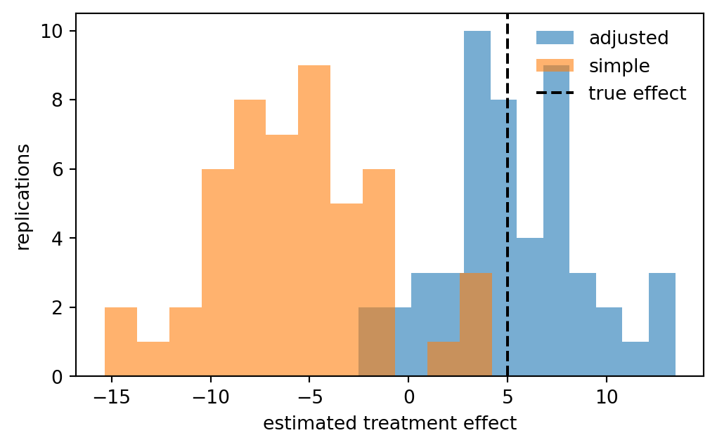
In the biased design, the unadjusted comparison is pulled downward because treated students tend to have lower pre-test scores. Conditioning on the pre-test moves the estimate back toward the true 5-point effect and usually improves precision.