# Earnings regression
Source: `Earnings/earnings_regression.Rmd`
The original page studies several regressions of annual earnings on height and sex: first on the dollar scale, then on log-earnings, with posterior predictive checks. This Python port keeps `statsmodels` for familiar least-squares summaries and uses the lightweight Bayesian linear-regression helper for posterior and posterior-predictive draws.
## Setup and data
```{python}
from pathlib import Path
import numpy as np
import pandas as pd
import matplotlib.pyplot as plt
import statsmodels.formula.api as smf
from scipy.stats import gaussian_kde
from python.bayes_glm import bayes_lm

root = Path("../../ROS-Examples")
earnings = pd.read_csv(root / "Earnings/data/earnings.csv")
rng = np.random.default_rng(7783)
earnings["height_jitter"] = earnings["height"] + rng.uniform(-0.2, 0.2, len(earnings))
earnings.head()
```
```{python}
earnings[["height", "male", "earn", "earnk", "age", "education"]].describe()
```
## Normal linear regression on dollars
```{python}
fit_0 = smf.ols("earn ~ height", data=earnings).fit()
fit_0_bayes = bayes_lm("earn ~ height", data=earnings, draws=1000, prior_scale=10.0, seed=7783)
fit_0.summary()
```
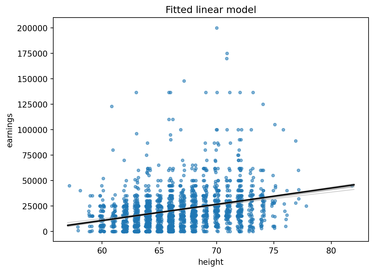
```{python}
sims_0 = fit_0_bayes.beta_draws
keep = earnings["earn"] <= 200_000
xs = np.linspace(earnings.height.min(), earnings.height.max(), 200)

fig, ax = plt.subplots()
ax.scatter(earnings.loc[keep, "height_jitter"], earnings.loc[keep, "earn"], s=12, alpha=0.55)
for b in sims_0[:10]:
    ax.plot(xs, b[0] + b[1] * xs, color="gray", alpha=0.45, linewidth=0.8)
ax.plot(xs, fit_0.params["Intercept"] + fit_0.params["height"] * xs, color="black")
ax.set_xlabel("height")
ax.set_ylabel("earnings")
ax.set_title("Fitted linear model")
```
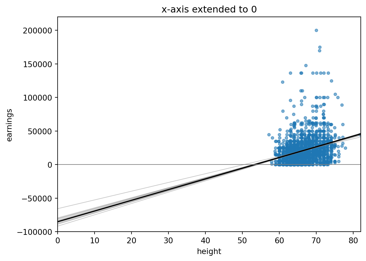
The intercept is not meaningful: the model is being extrapolated to height zero. That is the point of the next display.
```{python}
fig, ax = plt.subplots()
ax.scatter(earnings.loc[keep, "height_jitter"], earnings.loc[keep, "earn"], s=12, alpha=0.55)
for b in sims_0[:10]:
    ax.plot(np.linspace(0, earnings.height.max(), 200), b[0] + b[1] * np.linspace(0, earnings.height.max(), 200), color="gray", alpha=0.45, linewidth=0.8)
ax.plot(np.linspace(0, earnings.height.max(), 200), fit_0.params["Intercept"] + fit_0.params["height"] * np.linspace(0, earnings.height.max(), 200), color="black")
ax.axhline(0, color="gray", linewidth=0.8)
ax.set_xlim(0, earnings.height.max())
ax.set_ylim(-100_000, 220_000)
ax.set_xlabel("height")
ax.set_ylabel("earnings")
ax.set_title("x-axis extended to 0")
```
## Earnings in thousands of dollars
Scaling the outcome rescales the coefficients but does not otherwise change the fitted values.
```{python}
fit_1 = smf.ols("earnk ~ height", data=earnings).fit()
pd.DataFrame({
    "dollar_model": fit_0.params,
    "thousand_model_times_1000": fit_1.params * 1000,
})
```
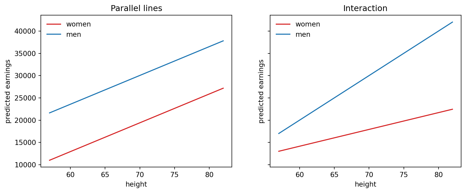
## Add sex indicator and interaction
```{python}
fit_2 = smf.ols("earnk ~ height + male", data=earnings).fit()
fit_3 = smf.ols("earnk ~ height * male", data=earnings).fit()
fit_2.summary()
```
```{python}
fit_3.summary()
```
```{python}
coef2 = fit_2.params * 1000
coef3 = fit_3.params * 1000
xgrid = np.linspace(earnings.height.min(), earnings.height.max(), 200)

fig, axes = plt.subplots(1, 2, figsize=(11, 4), sharey=True)
axes[0].plot(xgrid, coef2["Intercept"] + coef2["height"] * xgrid, color="tab:red", label="women")
axes[0].plot(xgrid, coef2["Intercept"] + coef2["male"] + coef2["height"] * xgrid, color="tab:blue", label="men")
axes[0].set_title("Parallel lines")

axes[1].plot(xgrid, coef3["Intercept"] + coef3["height"] * xgrid, color="tab:red", label="women")
axes[1].plot(xgrid, coef3["Intercept"] + coef3["male"] + (coef3["height"] + coef3["height:male"]) * xgrid, color="tab:blue", label="men")
axes[1].set_title("Interaction")

for ax in axes:
    ax.set_xlabel("height")
    ax.set_ylabel("predicted earnings")
    ax.legend(frameon=False)
```
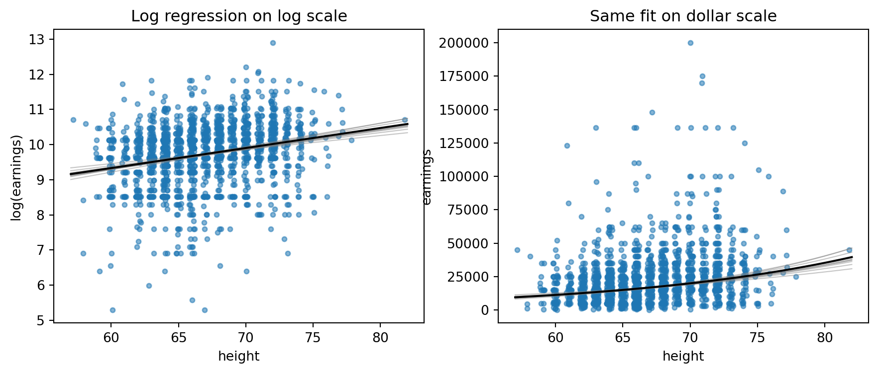
## Log earnings models
The dollar-scale normal model is a poor match for a strongly skewed outcome with many low values. The R page therefore compares models for `log(earn)` among respondents with positive earnings.
```{python}
pos = earnings[earnings.earn > 0].copy()
pos["log_earn"] = np.log(pos["earn"])
pos["log10_earn"] = np.log10(pos["earn"])
pos["log_height"] = np.log(pos["height"])
pos["z_height"] = (pos["height"] - pos["height"].mean()) / pos["height"].std()

logmodel_1 = smf.ols("log_earn ~ height", data=pos).fit()
logmodel_1_bayes = bayes_lm("log_earn ~ height", data=pos, draws=1000, prior_scale=10.0, seed=7784)
log10model_1 = smf.ols("log10_earn ~ height", data=pos).fit()
logmodel_2 = smf.ols("log_earn ~ height + male", data=pos).fit()
loglogmodel_2 = smf.ols("log_earn ~ log_height + male", data=pos).fit()
logmodel_3 = smf.ols("log_earn ~ height * male", data=pos).fit()
logmodel_3a = smf.ols("log_earn ~ z_height * male", data=pos).fit()

pd.DataFrame({
    "log height": logmodel_1.params,
    "log height+male": logmodel_2.params,
}).round(3)
```
```{python}
sims_log = logmodel_1_bayes.beta_draws
xs = np.linspace(pos.height.min(), pos.height.max(), 200)
fig, axes = plt.subplots(1, 2, figsize=(11, 4))

axes[0].scatter(pos.height_jitter, pos.log_earn, s=12, alpha=0.55)
for b in sims_log[:10]:
    axes[0].plot(xs, b[0] + b[1] * xs, color="gray", alpha=0.45, linewidth=0.8)
axes[0].plot(xs, logmodel_1.params["Intercept"] + logmodel_1.params["height"] * xs, color="black")
axes[0].set_xlabel("height")
axes[0].set_ylabel("log(earnings)")
axes[0].set_title("Log regression on log scale")

small = pos[pos.earn <= 200_000]
axes[1].scatter(small.height_jitter, small.earn, s=12, alpha=0.55)
for b in sims_log[:10]:
    axes[1].plot(xs, np.exp(b[0] + b[1] * xs), color="gray", alpha=0.45, linewidth=0.8)
axes[1].plot(xs, np.exp(logmodel_1.params["Intercept"] + logmodel_1.params["height"] * xs), color="black")
axes[1].set_xlabel("height")
axes[1].set_ylabel("earnings")
axes[1].set_title("Same fit on dollar scale")
```
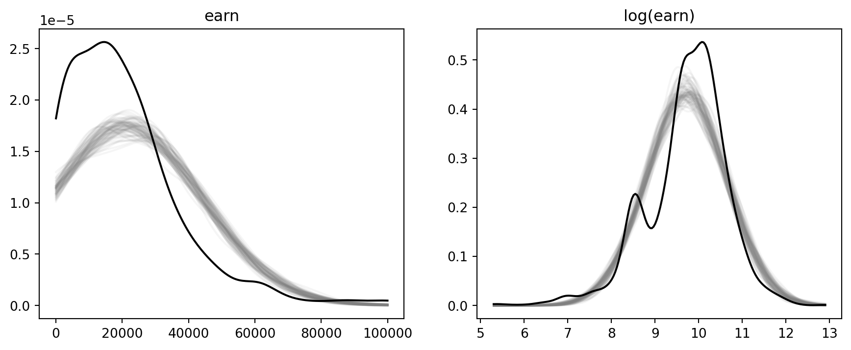
## Lightweight posterior predictive checks
The Bayesian helper supplies a direct analogue of `posterior_predict()`: draw coefficients and residual scale from the Gaussian linear-model posterior, then draw replicated outcomes.
```{python}
yrep_0 = fit_0_bayes.predict(seed=1)[:200]
yrep_log_1 = logmodel_1_bayes.predict(seed=2)[:200]

fig, axes = plt.subplots(1, 2, figsize=(11, 4))
for draw in yrep_0[:80]:
    kde = gaussian_kde(draw)
    grid = np.linspace(np.percentile(earnings.earn, 1), np.percentile(earnings.earn, 99), 200)
    axes[0].plot(grid, kde(grid), color="gray", alpha=0.08)
axes[0].plot(grid, gaussian_kde(earnings.earn)(grid), color="black")
axes[0].set_title("earn")

log_grid = np.linspace(pos.log_earn.min(), pos.log_earn.max(), 200)
for draw in yrep_log_1[:80]:
    kde = gaussian_kde(draw)
    axes[1].plot(log_grid, kde(log_grid), color="gray", alpha=0.08)
axes[1].plot(log_grid, gaussian_kde(pos.log_earn)(log_grid), color="black")
axes[1].set_title("log(earn)")
```
## CmdStanPy analogue
```{python}
#| eval: false
from cmdstanpy import CmdStanModel

stan_code = """
data {
  int<lower=1> N;
  matrix[N, 3] X;
  vector[N] y;
}
parameters {
  vector[3] beta;
  real<lower=0> sigma;
}
model {
  beta ~ normal(0, 10);
  sigma ~ exponential(1);
  y ~ normal(X * beta, sigma);
}
generated quantities {
  vector[N] y_rep;
  for (n in 1:N) y_rep[n] = normal_rng(dot_product(row(X, n), beta), sigma);
}
"""
Path("earnings_height_male.stan").write_text(stan_code)
X = np.column_stack([np.ones(len(pos)), pos.height.to_numpy(), pos.male.to_numpy()])
model = CmdStanModel(stan_file="earnings_height_male.stan")
fit = model.sample(data={"N": len(pos), "X": X, "y": pos.log_earn.to_numpy()}, seed=7783)
fit.summary().loc[["beta[1]", "beta[2]", "beta[3]", "sigma"]]
```