# Arsenic wells: building logistic models by optimization
Source: `Arsenic/arsenic_logistic_building_optimizing.Rmd`
The R page uses `stan_glm(..., algorithm='optimizing')`, which returns a posterior mode rather than full MCMC draws. The Python port keeps the model path Bayesian and formula-first with `lapylace`; where the source page draws fitted curves, we use posterior draws from the same Bernoulli-logit formulas.
## Setup and data
```{python}
from pathlib import Path
import numpy as np
import pandas as pd
import matplotlib.pyplot as plt
import lapylace as lp
from scipy.special import expit
from scipy.stats import norm

root = Path("../../ROS-Examples")
wells = pd.read_csv(root / "Arsenic/data/wells.csv")
wells["y"] = wells["switch"]
wells["dist100"] = wells["dist"] / 100
wells["educ4"] = wells["educ"] / 4
wells.head()
```
## Null-model log scores
```{python}
y = wells["y"].to_numpy()
def bernoulli_log_score(p, y=y):
    p = np.clip(p, 1e-12, 1 - 1e-12)
    return float(np.sum(y * np.log(p) + (1 - y) * np.log(1 - p)))

pd.Series({
    "coin flip": bernoulli_log_score(0.5),
    "intercept only": bernoulli_log_score(y.mean()),
}).round(1)
```
## Model helpers
```{python}
def fit_logit(formula, seed):
    return lp.stan_glm(
        formula,
        data=wells,
        family=lp.bernoulli(),
        prior=lp.normal(0, 2.5),
        prior_intercept=lp.normal(0, 5),
        chains=4,
        parallel_chains=4,
        iter_warmup=500,
        iter_sampling=1000,
        seed=seed,
        refresh=100,
    )

def coef_draws(fit):
    return np.column_stack([fit.alpha_draws(), fit.beta_draws()])

def coef_medians(fit):
    return pd.Series(np.median(coef_draws(fit), axis=0), index=["Intercept", *fit.columns])

def summarize_fit(fit):
    draws = coef_draws(fit)
    coef = np.median(draws, axis=0)
    se = np.std(draws, axis=0)
    return pd.DataFrame({"coef": coef, "se": se, "z": coef / se}, index=["Intercept", *fit.columns]).round(3)

def predict_prob(fit, data=wells):
    return fit.posterior_epred(data).mean(axis=0)

def in_sample_log_score(fit):
    return bernoulli_log_score(predict_prob(fit))

def jitter_binary(a, seed=123, jitt=0.05):
    rng = np.random.default_rng(seed)
    a = np.asarray(a)
    return a + (1 - 2 * a) * rng.uniform(0, jitt, size=len(a))
```
## A single predictor: distance
```{python}
fit_1 = fit_logit("y ~ dist", seed=15401)
fit_2 = fit_logit("y ~ dist100", seed=15402)
summarize_fit(fit_2)
```
```{python}
pd.Series({
    "dist, meters": in_sample_log_score(fit_1),
    "dist, hundreds of meters": in_sample_log_score(fit_2),
}).round(1)
```
```{python}
fig, ax = plt.subplots(figsize=(5, 4))
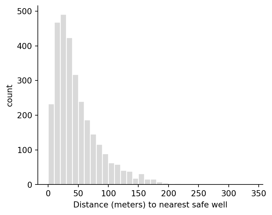
ax.hist(wells["dist"], bins=np.arange(0, wells["dist"].max() + 10, 10), color="0.85", edgecolor="white")
ax.set(xlabel="Distance (meters) to nearest safe well", ylabel="count")
ax.spines[["top", "right"]].set_visible(False)
```
```{python}
xs = np.linspace(0, wells["dist"].max(), 300)
y_jit = jitter_binary(y)
coef_2 = coef_medians(fit_2)
fig, ax = plt.subplots(figsize=(5, 4))
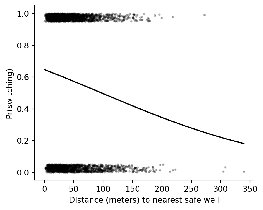
ax.scatter(wells["dist"], y_jit, s=4, color="black", alpha=0.25)
ax.plot(xs, expit(coef_2["Intercept"] + coef_2["dist100"] * xs / 100), color="black")
ax.set(xlabel="Distance (meters) to nearest safe well", ylabel="Pr(switching)")
ax.spines[["top", "right"]].set_visible(False)
```
### Approximate coefficient and prediction uncertainty
```{python}
rng = np.random.default_rng(2024)
fit_2_draws = coef_draws(fit_2)
fit_2_draws[:5]
```
```{python}
fig, ax = plt.subplots(figsize=(4, 4))
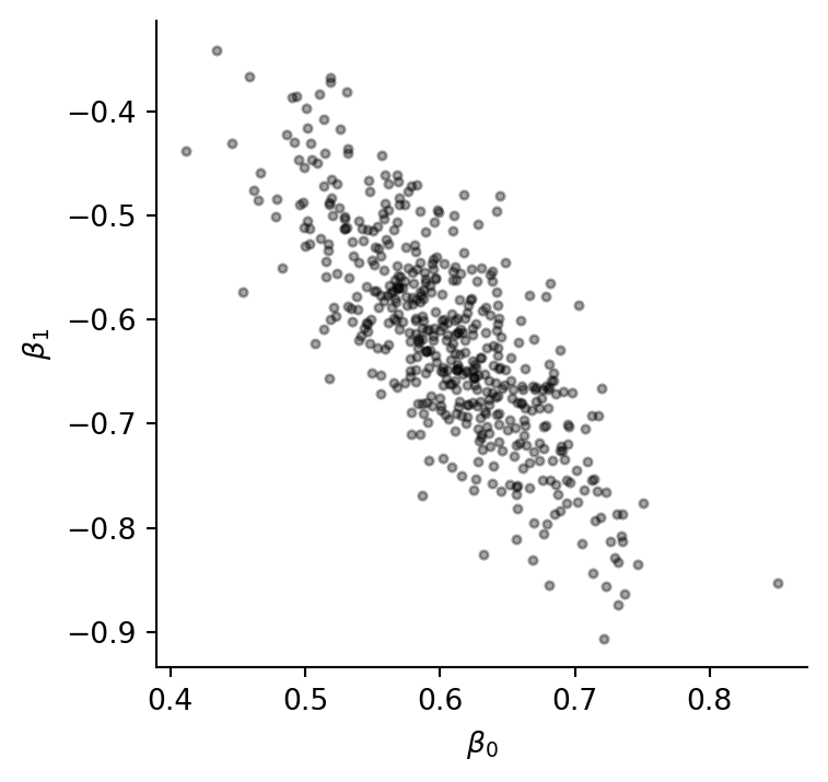
ax.scatter(fit_2_draws[:, 0], fit_2_draws[:, 1], s=8, color="black", alpha=0.35)
ax.set(xlabel=r"$\beta_0$", ylabel=r"$\beta_1$")
ax.spines[["top", "right"]].set_visible(False)
```
```{python}
fig, ax = plt.subplots(figsize=(5, 4))
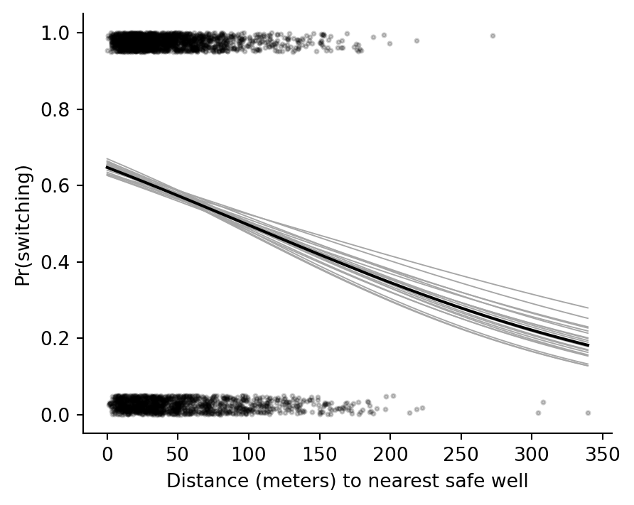
ax.scatter(wells["dist"], y_jit, s=4, color="black", alpha=0.20)
for b0, b1 in fit_2_draws[:20]:
    ax.plot(xs, expit(b0 + b1 * xs / 100), color="0.65", lw=0.7)
ax.plot(xs, expit(coef_2["Intercept"] + coef_2["dist100"] * xs / 100), color="black")
ax.set(xlabel="Distance (meters) to nearest safe well", ylabel="Pr(switching)")
ax.spines[["top", "right"]].set_visible(False)
```
## Two predictors: distance and arsenic
```{python}
fig, ax = plt.subplots(figsize=(5, 4))
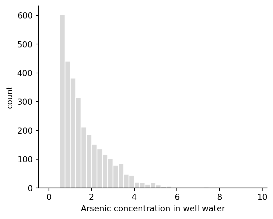
ax.hist(wells["arsenic"], bins=np.arange(0, wells["arsenic"].max() + 0.25, 0.25), color="0.85", edgecolor="white")
ax.set(xlabel="Arsenic concentration in well water", ylabel="count")
ax.spines[["top", "right"]].set_visible(False)
```
```{python}
fit_3 = fit_logit("y ~ dist100 + arsenic", seed=15403)
summarize_fit(fit_3)
```
```{python}
pd.Series({"dist100": in_sample_log_score(fit_2), "dist100 + arsenic": in_sample_log_score(fit_3)}).round(1)
```
```{python}
pred2 = predict_prob(fit_2)
pred3 = predict_prob(fit_3)
improvement_23 = np.r_[pred3[y == 1] - pred2[y == 1], pred2[y == 0] - pred3[y == 0]].mean()
round(float(improvement_23), 3)
```
```{python}
fig, ax = plt.subplots(figsize=(5, 4))
ax.scatter(wells["dist"], y_jit, s=4, color="black", alpha=0.2)
coef_3 = coef_medians(fit_3)
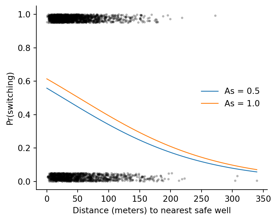
for a, label in [(0.5, "As = 0.5"), (1.0, "As = 1.0")]:
    p = expit(coef_3["Intercept"] + coef_3["dist100"] * xs / 100 + coef_3["arsenic"] * a)
    ax.plot(xs, p, lw=1, label=label)
ax.set(xlabel="Distance (meters) to nearest safe well", ylabel="Pr(switching)")
ax.legend(frameon=False)
ax.spines[["top", "right"]].set_visible(False)
```
## Interaction and centering
```{python}
fit_4 = fit_logit("y ~ dist100 * arsenic", seed=15404)
wells["c_dist100"] = wells["dist100"] - wells["dist100"].mean()
wells["c_arsenic"] = wells["arsenic"] - wells["arsenic"].mean()
fit_5 = fit_logit("y ~ c_dist100 * c_arsenic", seed=15405)
summarize_fit(fit_4)
```
Centering changes the interpretation and numerical stability of the intercept and main effects; it does not change fitted probabilities for this interaction surface.
```{python}
np.max(np.abs(predict_prob(fit_4) - predict_prob(fit_5)))
```
## Social predictors and education interactions
```{python}
fit_6 = fit_logit("y ~ dist100 + arsenic + educ4 + assoc", seed=15406)
fit_7 = fit_logit("y ~ dist100 + arsenic + educ4", seed=15407)
wells["c_educ4"] = wells["educ4"] - wells["educ4"].mean()
fit_8 = fit_logit("y ~ c_dist100 + c_arsenic + c_educ4 + c_dist100:c_educ4 + c_arsenic:c_educ4", seed=15408)
pd.concat({
    "with association": summarize_fit(fit_6)["coef"],
    "without association": summarize_fit(fit_7)["coef"],
    "education interactions": summarize_fit(fit_8)["coef"],
}, axis=1).round(2)
```
```{python}
scores = pd.Series({
    "dist100 + arsenic": in_sample_log_score(fit_3),
    "+ interaction": in_sample_log_score(fit_4),
    "+ educ4 + assoc": in_sample_log_score(fit_6),
    "+ educ4": in_sample_log_score(fit_7),
    "+ education interactions": in_sample_log_score(fit_8),
})
scores.round(1)
```
```{python}
pred8 = predict_prob(fit_8)
improvement_38 = np.r_[pred8[y == 1] - pred3[y == 1], pred3[y == 0] - pred8[y == 0]].mean()
round(float(improvement_38), 3)
```
## Log transform of arsenic
```{python}
wells["log_arsenic"] = np.log(wells["arsenic"])
wells["c_log_arsenic"] = wells["log_arsenic"] - wells["log_arsenic"].mean()
fit_3a = fit_logit("y ~ dist100 + log_arsenic", seed=15409)
fit_4a = fit_logit("y ~ dist100 * log_arsenic", seed=15410)
fit_8a = fit_logit("y ~ c_dist100 + c_log_arsenic + c_educ4 + c_dist100:c_educ4 + c_log_arsenic:c_educ4", seed=15411)
pd.Series({
    "dist100 + arsenic": in_sample_log_score(fit_3),
    "dist100 + log(arsenic)": in_sample_log_score(fit_3a),
    "+ log interaction": in_sample_log_score(fit_4a),
    "+ log arsenic education interactions": in_sample_log_score(fit_8a),
}).round(1)
```
## Leave-one-out note
The R source reports PSIS-LOO via `loo()` for the fitted `stan_glm` objects. The `lapylace` fits expose the same ArviZ path with `fit.to_arviz()` and `fit.loo()`; the in-sample log scores above are kept only as quick checks of the model-building sequence.
Social predictors and education interactions