import os, sys

import arviz as az
import numpy as np
import pandas as pd

# import stan interface
from cmdstanpy import CmdStanModel

# add utilities directory to path
# so we can import check_utility
util_path = os.path.abspath(os.path.join(os.path.pardir, 'utilities_and_data'))
if util_path not in sys.path and os.path.exists(util_path):
    sys.path.insert(0, util_path)
from check_utility import check_div, check_energy, check_treedepth

az.style.use('arviz-white')Bayesian Logistic Regression with CmdStanPy
TODO: Work in progress
Authors: Jonah Gabry, Ben Goodrich, Aki Vehtari, Tuomas Sivula
The introduction to Bayesian logistic regression is from a CRAN vignette by Jonah Gabry and Ben Goodrich. CRAN vignette was modified to a R notebook by Aki Vehtari. Instead of wells data in CRAN vignette, Pima Indians data is used. The end of the notebook differs significantly from the CRAN vignette. The R notebook was ported to this Python notebook by Aki Vehtari and Tuomas Sivula.
Introduction
This vignette explains how to estimate generalized linear models (GLMs) for binary (Bernoulli) response variables using CmdStanPy.
The four steps of a Bayesian analysis are
- Specify a joint distribution for the outcome(s) and all the unknowns, which typically takes the form of a marginal prior distribution for the unknowns multiplied by a likelihood for the outcome(s) conditional on the unknowns. This joint distribution is proportional to a posterior distribution of the unknowns conditional on the observed data
- Draw from posterior distribution using Markov Chain Monte Carlo (MCMC).
- Evaluate how well the model fits the data and possibly revise the model.
- Draw from the posterior predictive distribution of the outcome(s) given interesting values of the predictors in order to visualize how a manipulation of a predictor affects (a function of) the outcome(s). This notebook demonstrates Steps 1-3 when the likelihood is the product of conditionally independent binomial distributions (possibly with only one trial per observation).
Likelihood
For a binomial GLM the likelihood for one observation \(y\) can be written as a conditionally binomial PMF \[\binom{n}{y} \pi^{y} (1 - \pi)^{n - y},\] where \(n\) is the known number of trials, \(\pi = g^{-1}(\eta)\) is the probability of success and \(\eta = \alpha + \mathbf{x}^\top \boldsymbol{\beta}\) is a linear predictor. For a sample of size \(N\), the likelihood of the entire sample is the product of \(N\) individual likelihood contributions.
Because \(\pi\) is a probability, for a binomial model the link function \(g\) maps between the unit interval (the support of \(\pi\)) and the set of all real numbers \(\mathbb{R}\). When applied to a linear predictor \(\eta\) with values in \(\mathbb{R}\), the inverse link function \(g^{-1}(\eta)\) therefore returns a valid probability between 0 and 1.
The two most common link functions used for binomial GLMs are the logit and probit functions. With the logit (or log-odds) link function \(g(x) = \ln{\left(\frac{x}{1-x}\right)}\), the likelihood for a single observation becomes
\[\binom{n}{y}\left(\text{logit}^{-1}(\eta)\right)^y \left(1 - \text{logit}^{-1}(\eta)\right)^{n-y} = \binom{n}{y} \left(\frac{e^{\eta}}{1 + e^{\eta}}\right)^{y} \left(\frac{1}{1 + e^{\eta}}\right)^{n - y}\]
and the probit link function \(g(x) = \Phi^{-1}(x)\) yields the likelihood
\[\binom{n}{y} \left(\Phi(\eta)\right)^{y} \left(1 - \Phi(\eta)\right)^{n - y},\]
where \(\Phi\) is the CDF of the standard normal distribution. The differences between the logit and probit functions are minor and – if, as rstanarm does by default, the probit is scaled so its slope at the origin matches the logit’s – the two link functions should yield similar results. Unless the user has a specific reason to prefer the probit link, we recommend the logit simply because it will be slightly faster and more numerically stable.
In theory, there are infinitely many possible link functions, although in practice only a few are typically used.
Priors
A full Bayesian analysis requires specifying prior distributions \(f(\alpha)\) and \(f(\boldsymbol{\beta})\) for the intercept and vector of regression coefficients.
As an example, suppose we have \(K\) predictors and believe — prior to seeing the data — that \(\alpha, \beta_1, \dots, \beta_K\) are as likely to be positive as they are to be negative, but are highly unlikely to be far from zero. These beliefs can be represented by normal distributions with mean zero and a small scale (standard deviation).
If, on the other hand, we have less a priori confidence that the parameters will be close to zero then we could use a larger scale for the normal distribution and/or a distribution with heavier tails than the normal like the Student’s \(t\) distribution.
Posterior
With independent prior distributions, the joint posterior distribution for \(\alpha\) and \(\boldsymbol{\beta}\) is proportional to the product of the priors and the \(N\) likelihood contributions:
\[f\left(\alpha,\boldsymbol{\beta} | \mathbf{y},\mathbf{X}\right) \propto f\left(\alpha\right) \times \prod_{k=1}^K f\left(\beta_k\right) \times \prod_{i=1}^N { g^{-1}\left(\eta_i\right)^{y_i} \left(1 - g^{-1}\left(\eta_i\right)\right)^{n_i-y_i}}.\]
This is posterior distribution that CmdStanPy will draw from when using MCMC.
Logistic Regression Example
When the logit link function is used the model is often referred to as a logistic regression model (the inverse logit function is the CDF of the standard logistic distribution). As an example, here we will show how to carry out a analysis for Pima Indians data set similar to analysis from Chapter 5.4 of Gelman and Hill (2007) using CmdStanPy.
Data
First we load and pre-process data.
# load data
data_path = os.path.abspath(
    os.path.join(
        os.path.pardir,
        'utilities_and_data',
        'diabetes.csv'
    )
)
data = pd.read_csv(data_path)
# print some basic info()
data.info()
<class 'pandas.core.frame.DataFrame'>
RangeIndex: 768 entries, 0 to 767
Data columns (total 9 columns):
# Column Non-Null Count Dtype
--- ------ -------------- -----
0 Pregnancies 768 non-null int64
1 Glucose 768 non-null int64
2 BloodPressure 768 non-null int64
3 SkinThickness 768 non-null int64
4 Insulin 768 non-null int64
5 BMI 768 non-null float64
6 DiabetesPedigreeFunction 768 non-null float64
7 Age 768 non-null int64
8 Outcome 768 non-null int64
dtypes: float64(2), int64(7)
memory usage: 54.1 KB# preview some first rows
data.head()| Pregnancies | Glucose | BloodPressure | SkinThickness | Insulin | BMI | DiabetesPedigreeFunction | Age | Outcome | |
|---|---|---|---|---|---|---|---|---|---|
| 0 | 6 | 148 | 72 | 35 | 0 | 33.6 | 0.627 | 50 | 1 |
| 1 | 1 | 85 | 66 | 29 | 0 | 26.6 | 0.351 | 31 | 0 |
| 2 | 8 | 183 | 64 | 0 | 0 | 23.3 | 0.672 | 32 | 1 |
| 3 | 1 | 89 | 66 | 23 | 94 | 28.1 | 0.167 | 21 | 0 |
| 4 | 0 | 137 | 40 | 35 | 168 | 43.1 | 2.288 | 33 | 1 |
# some summary
data.describe()| Pregnancies | Glucose | BloodPressure | SkinThickness | Insulin | BMI | DiabetesPedigreeFunction | Age | Outcome | |
|---|---|---|---|---|---|---|---|---|---|
| count | 768.000000 | 768.000000 | 768.000000 | 768.000000 | 768.000000 | 768.000000 | 768.000000 | 768.000000 | 768.000000 |
| mean | 3.845052 | 120.894531 | 69.105469 | 20.536458 | 79.799479 | 31.992578 | 0.471876 | 33.240885 | 0.348958 |
| std | 3.369578 | 31.972618 | 19.355807 | 15.952218 | 115.244002 | 7.884160 | 0.331329 | 11.760232 | 0.476951 |
| min | 0.000000 | 0.000000 | 0.000000 | 0.000000 | 0.000000 | 0.000000 | 0.078000 | 21.000000 | 0.000000 |
| 25% | 1.000000 | 99.000000 | 62.000000 | 0.000000 | 0.000000 | 27.300000 | 0.243750 | 24.000000 | 0.000000 |
| 50% | 3.000000 | 117.000000 | 72.000000 | 23.000000 | 30.500000 | 32.000000 | 0.372500 | 29.000000 | 0.000000 |
| 75% | 6.000000 | 140.250000 | 80.000000 | 32.000000 | 127.250000 | 36.600000 | 0.626250 | 41.000000 | 1.000000 |
| max | 17.000000 | 199.000000 | 122.000000 | 99.000000 | 846.000000 | 67.100000 | 2.420000 | 81.000000 | 1.000000 |
Preprocess data
# modify the data column names slightly for easier typing
# rename DiabetesPedigreeFunction to dpf
data.rename(columns={'DiabetesPedigreeFunction': 'dpf'}, inplace=True)
# make lower
data.rename(columns=lambda old_name: old_name.lower(), inplace=True)
# removing those observation rows with 0 in selected variables
normed_predictors = [
'glucose',
'bloodpressure',
'skinthickness',
'insulin',
'bmi'
]
data = data[(data[normed_predictors] != 0).all(axis=1)]# scale the covariates for easier comparison of coefficient posteriors
# N.B. int columns turn into floats
data.iloc[:,:-1] -= data.iloc[:,:-1].mean()
data.iloc[:,:-1] /= data.iloc[:,:-1].std()# preview some first rows againg
data.head()| pregnancies | glucose | bloodpressure | skinthickness | insulin | bmi | dpf | age | outcome | |
|---|---|---|---|---|---|---|---|---|---|
| 3 | -0.716511 | -1.089653 | -0.373178 | -0.584363 | -0.522175 | -0.709514 | -1.030559 | -0.967063 | 0 |
| 4 | -1.027899 | 0.465719 | -2.453828 | 0.556709 | 0.100502 | 1.424909 | 5.108582 | 0.209318 | 1 |
| 6 | -0.093734 | -1.446093 | -1.653578 | 0.271441 | -0.572662 | -0.296859 | -0.796108 | -0.476904 | 1 |
| 8 | -0.405123 | 2.409934 | -0.053078 | 1.507603 | 3.255961 | -0.368007 | -1.056609 | 2.169953 | 1 |
| 13 | -0.716511 | 2.150705 | -0.853328 | -0.584363 | 5.805571 | -0.424924 | -0.361940 | 2.758143 | 1 |
# preparing the inputs
X = data.iloc[:,:-1]
y = data.iloc[:,-1]
# get shape into variables
n, p = X.shape
print('number of observations = {}'.format(n))
print('number of predictors = {}'.format(p))number of observations = 392
number of predictors = 8Stan model code for logistic regression
Logistic regression with Student’s \(t\) prior as discussed above.
with open('logistic_t.stan') as file:
    print(file.read())
/**
* Logistic regression t-prior
*
* Priors:
* weights - student t
* intercept - student t
*/
data {
int<lower=0> n; // number of data points
int<lower=1> d; // explanatory variable dimension
matrix[n, d] X; // explanatory variable
array[n] int<lower=0, upper=1> y; // response variable
int<lower=1> p_alpha_df; // prior degrees of freedom for alpha
real p_alpha_loc; // prior location for alpha
real<lower=0> p_alpha_scale; // prior scale for alpha
int<lower=1> p_beta_df; // prior degrees of freedom for beta
real p_beta_loc; // prior location for beta
real<lower=0> p_beta_scale; // prior scale for beta
}
parameters {
real alpha; // intercept
vector[d] beta; // explanatory variable weights
}
transformed parameters {
// linear predictor
vector[n] eta;
eta = alpha + X * beta;
}
model {
alpha ~ student_t(p_alpha_df, p_alpha_loc, p_alpha_scale);
beta ~ student_t(p_beta_df, p_beta_loc, p_beta_scale);
y ~ bernoulli_logit(eta);
}
generated quantities {
vector[n] log_lik;
for (i in 1:n)
log_lik[i] = bernoulli_logit_lpmf(y[i] | eta[i]);
}
model = CmdStanModel(stan_file='logistic_t.stan')Set priors and sample from the posterior
Here we’ll use a Student t prior with 7 degrees of freedom and a scale of 2.5, which, as discussed above, is a reasonable default prior when coefficients should be close to zero but have some chance of being large. CmdStanPy returns the posterior distribution for the parameters describing the uncertainty related to unknown parameter values.
data1 = dict(
    n=n,
    d=p,
    X=X,
    y=y,
    p_alpha_df=7,
    p_alpha_loc=0,
    p_alpha_scale=2.5,
    p_beta_df=7,
    p_beta_loc=0,
    p_beta_scale=2.5
)
fit1 = model.sample(data=data1, seed=74749)
idata_t = az.from_cmdstanpy(fit1)
Inspect the resulting posterior
Check n_effs and Rhats
az.summary(idata_t, var_names=['alpha', 'beta'], kind='diagnostics')| mcse_mean | mcse_sd | ess_bulk | ess_tail | r_hat | |
|---|---|---|---|---|---|
| alpha | 0.002 | 0.002 | 5029.0 | 3276.0 | 1.0 |
| beta[0] | 0.003 | 0.003 | 3530.0 | 3136.0 | 1.0 |
| beta[1] | 0.003 | 0.002 | 3995.0 | 3275.0 | 1.0 |
| beta[2] | 0.002 | 0.002 | 4834.0 | 3061.0 | 1.0 |
| beta[3] | 0.003 | 0.003 | 3456.0 | 2771.0 | 1.0 |
| beta[4] | 0.003 | 0.002 | 3753.0 | 3300.0 | 1.0 |
| beta[5] | 0.003 | 0.003 | 3277.0 | 2917.0 | 1.0 |
| beta[6] | 0.002 | 0.003 | 5797.0 | 3041.0 | 1.0 |
| beta[7] | 0.003 | 0.003 | 3151.0 | 3009.0 | 1.0 |
n_effs are high and Rhats<1.1, which is good.
Next we check divergences, E-BMFI and treedepth exceedences as explained in Robust Statistical Workflow with PyStan Case Study by Michael Betancourt.
check_div(idata_t)
check_energy(idata_t)
check_treedepth(idata_t)
We don’t get any warning message, so everything is fine based on these diagnostics and we can proceed with our analysis.
Visualise the marginal posterior distributions of each parameter
ax = az.plot_forest(idata_t,
               combined=True,
               var_names=['alpha', 'beta'],
               )
ax[0].axvline(0, color="C1", linestyle="dotted");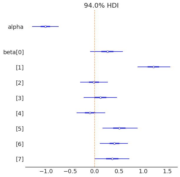
We can use Pareto smoothed importance sampling leave-one-out cross-validation to estimate the predictive performance.
loo_t = az.loo(idata_t)
loo_t
Computed from 4000 posterior samples and 392 observations log-likelihood matrix.
Estimate SE
elpd_loo -182.33 11.99
p_loo 10.98 -
------
Pareto k diagnostic values:
Count Pct.
(-Inf, 0.70] (good) 392 100.0%
(0.70, 1] (bad) 0 0.0%
(1, Inf) (very bad) 0 0.0%Alternative horseshoe prior on weights
In this example, with \(n \gg p\) the difference is small, and thus we don’t expect much difference with a different prior and horseshoe prior is usually more useful for \(n<p\).
The global scale parameter for horseshoe prior is chosen as recommended by Juho Piironen and Aki Vehtari (2017). On the Hyperprior Choice for the Global Shrinkage Parameter in the Horseshoe Prior. Journal of Machine Learning Research: Workshop and Conference Proceedings (AISTATS 2017 Proceedings), accepted for publication. arXiv preprint arXiv:1610.05559.
with open('logistic_hs.stan') as file:
    print(file.read())
/**
* Logistic regression HS-prior
*
* Priors:
* weights - hierarchical shrinkage
* intercept - student t
*/
data {
int<lower=0> n; // number of data points
int<lower=1> d; // explanatory variable dimension
matrix[n, d] X; // explanatory variable
array[n] int<lower=0, upper=1> y; // response variable
int<lower=1> p_alpha_df; // prior alpha degrees of freedom
real p_alpha_loc; // prior alpha location
real<lower=0> p_alpha_scale; // prior scale alpha
int<lower=1> p_beta_df; // prior beta degrees of freedom
int<lower=1> p_beta_global_df; // prior beta global degrees of freedom
real<lower=0> p_beta_global_scale; // prior beta global scale
}
parameters {
// intercept
real alpha;
// auxiliary variables for the variance parameters
vector[d] z;
vector<lower=0>[d] lambda_r1;
vector<lower=0>[d] lambda_r2;
real<lower=0> tau_r1;
real<lower=0> tau_r2;
}
transformed parameters {
vector<lower=0>[d] lambda; // local variance parameter
real<lower=0> tau; // global variance parameter
vector[d] beta; // explanatory variable weights
vector[n] eta; // linear predictor
lambda = lambda_r1 .* sqrt(lambda_r2);
tau = tau_r1 * sqrt(tau_r2);
beta = z .* (lambda*tau);
eta = alpha + X * beta;
}
model {
// student t prior for intercept
alpha ~ student_t(p_alpha_df, p_alpha_loc, p_alpha_scale);
z ~ normal(0.0, 1.0);
// half t priors for lambdas
lambda_r1 ~ normal(0.0, 1.0);
lambda_r2 ~ inv_gamma(0.5*p_beta_df, 0.5*p_beta_df);
// half t priors for tau
tau_r1 ~ normal(0.0, p_beta_global_scale);
tau_r2 ~ inv_gamma(0.5*p_beta_global_df, 0.5*p_beta_global_df);
// observation model
y ~ bernoulli_logit(eta);
}
generated quantities {
vector[n] log_lik;
for (i in 1:n)
log_lik[i] = bernoulli_logit_lpmf(y[i] | eta[i]);
}
model = CmdStanModel(stan_file='logistic_hs.stan')p0 = 2 # prior guess for the number of relevant variables
tau0 = p0 / (p - p0) * 1 / np.sqrt(n)
data2 = dict(
n=n,
d=p,
X=X,
y=y,
p_alpha_df=7,
p_alpha_loc=0,
p_alpha_scale=2.5,
p_beta_df=1,
p_beta_global_df=1,
p_beta_global_scale=tau0
)
fit2 = model.sample(data=data2, seed=74749)
idata_hs = az.from_cmdstanpy(fit2) We see that the horseshoe prior has shrunk the posterior distribution of irrelevant features closer to zero, without affecting the posterior distribution of the relevant features.
az.summary(idata_hs, var_names=['alpha', 'beta'])| mean | sd | hdi_3% | hdi_97% | mcse_mean | mcse_sd | ess_bulk | ess_tail | r_hat | |
|---|---|---|---|---|---|---|---|---|---|
| alpha | -0.973 | 0.141 | -1.230 | -0.704 | 0.002 | 0.003 | 4363.0 | 2806.0 | 1.0 |
| beta[0] | 0.185 | 0.174 | -0.084 | 0.510 | 0.004 | 0.002 | 1592.0 | 2761.0 | 1.0 |
| beta[1] | 1.138 | 0.163 | 0.842 | 1.444 | 0.003 | 0.002 | 4221.0 | 3439.0 | 1.0 |
| beta[2] | 0.014 | 0.095 | -0.186 | 0.205 | 0.001 | 0.002 | 4643.0 | 3782.0 | 1.0 |
| beta[3] | 0.103 | 0.146 | -0.114 | 0.416 | 0.003 | 0.002 | 2547.0 | 3390.0 | 1.0 |
| beta[4] | -0.021 | 0.095 | -0.238 | 0.149 | 0.001 | 0.002 | 4373.0 | 3546.0 | 1.0 |
| beta[5] | 0.394 | 0.194 | -0.015 | 0.703 | 0.004 | 0.003 | 2170.0 | 1258.0 | 1.0 |
| beta[6] | 0.289 | 0.162 | -0.020 | 0.549 | 0.004 | 0.003 | 1733.0 | 1142.0 | 1.0 |
| beta[7] | 0.318 | 0.198 | -0.038 | 0.644 | 0.005 | 0.003 | 1778.0 | 1307.0 | 1.0 |
ax = az.plot_forest(idata_hs,
               combined=True,
               var_names=['alpha', 'beta'],
               )
ax[0].axvline(0, color="C1", linestyle="dotted");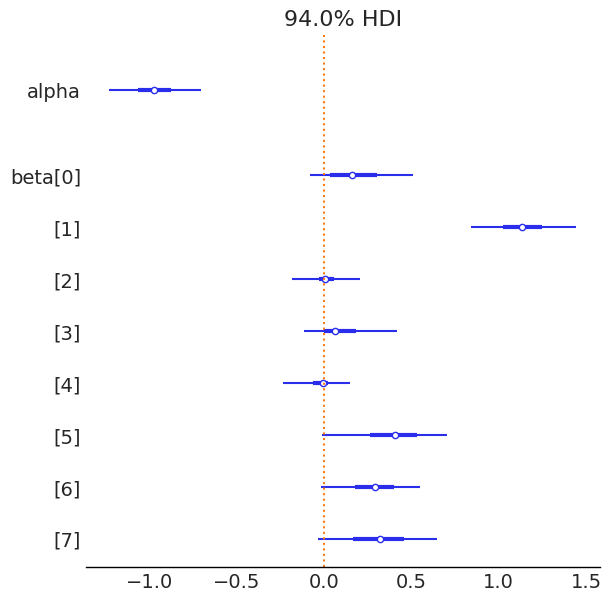
We compute LOO also for the model with Horseshoe prior. Expected log predictive density is higher, but not significantly. This is not surprising as this is a easy data with \(n \gg p\).
loo_hs = az.loo(idata_hs)
loo_hs
Computed from 4000 posterior samples and 392 observations log-likelihood matrix.
Estimate SE
elpd_loo -181.84 11.10
p_loo 9.47 -
------
Pareto k diagnostic values:
Count Pct.
(-Inf, 0.70] (good) 392 100.0%
(0.70, 1] (bad) 0 0.0%
(1, Inf) (very bad) 0 0.0%elpd_diff = loo_hs.loo_i - loo_t.loo_i
elpd_diff_se = np.sqrt(np.var(elpd_diff, ddof=1)*n)
elpd_diff = np.sum(elpd_diff)
print(f'elpd_diff: {elpd_diff:.4} (SE {elpd_diff_se:.3})')elpd_diff: 0.4864 (SE 1.53)