Annual earnings have a point mass at zero and a long right tail among people with positive earnings. The R example fits this as a two-part model: a logistic regression for whether earnings are positive, followed by a regression for log earnings conditional on positive earnings. This Python port uses lightweight Bayesian GLM helpers for the two fitted models and posterior predictive simulation.
Setup and data
Code
from pathlib import Pathimport numpy as npimport pandas as pdimport matplotlib.pyplot as pltfrom python.bayes_glm import bayes_lm, bayes_logitroot = Path("../../ROS-Examples")earnings = pd.read_csv(root /"Earnings/data/earnings.csv")earnings["positive_earn"] = (earnings["earn"] >0).astype(int)pos = earnings.loc[earnings["positive_earn"] ==1].copy()pos["log_earn"] = np.log(pos["earn"])rng = np.random.default_rng(15015)earnings.head()
The first model predicts the chance of being above zero. The second predicts the conditional distribution on the log scale for respondents whose earnings are positive.
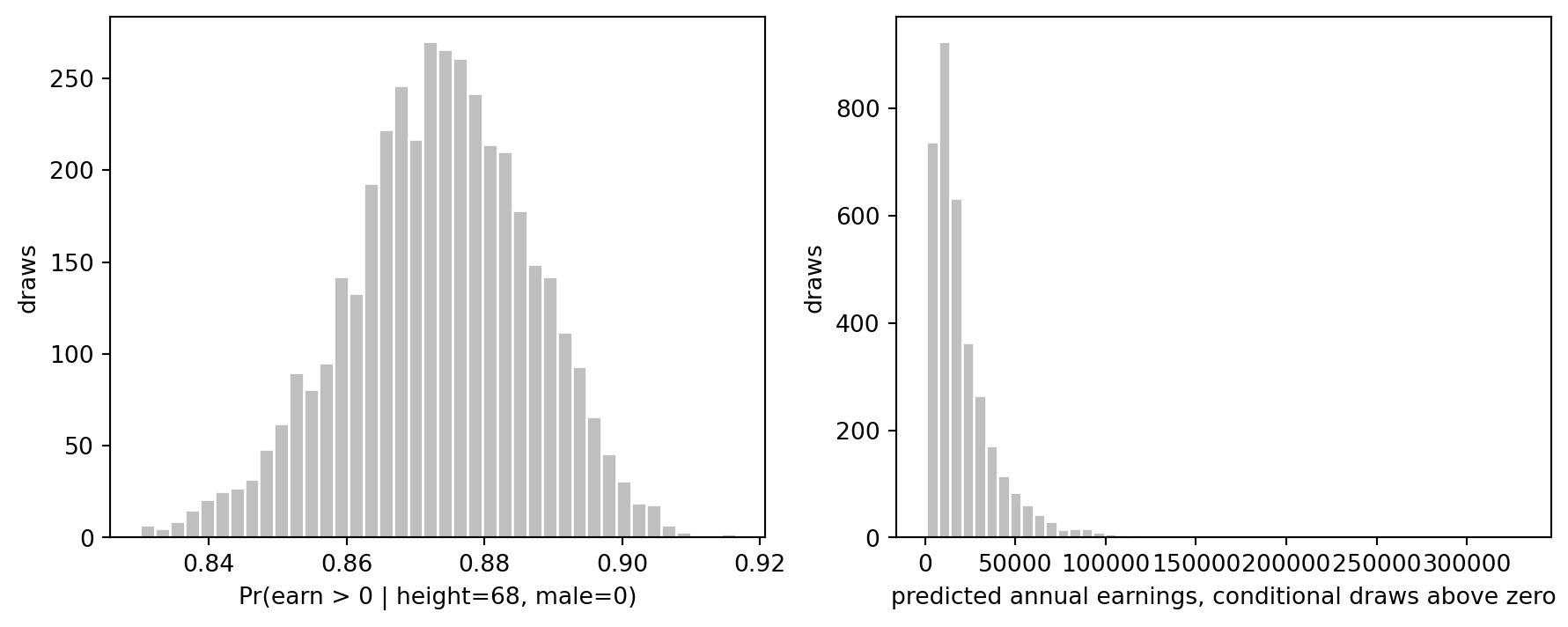
Predictions for a new person
The R page predicts earnings for a new person with height = 68 and male = 0. We reproduce the compound prediction by drawing coefficients for both models, drawing a Bernoulli indicator from the logistic part, and drawing log earnings from the normal linear model.
The compound model is more appropriate than a single normal regression on dollars because it separates the structural spike at zero from the skewed positive part of the distribution.
Source Code
# Earnings compound modelSource: `Earnings/earnings_compound.Rmd`Annual earnings have a point mass at zero and a long right tail among people with positive earnings. The R example fits this as a two-part model: a logistic regression for whether earnings are positive, followed by a regression for log earnings conditional on positive earnings. This Python port uses lightweight Bayesian GLM helpers for the two fitted models and posterior predictive simulation.## Setup and data```{python}from pathlib import Pathimport numpy as npimport pandas as pdimport matplotlib.pyplot as pltfrom python.bayes_glm import bayes_lm, bayes_logitroot = Path("../../ROS-Examples")earnings = pd.read_csv(root /"Earnings/data/earnings.csv")earnings["positive_earn"] = (earnings["earn"] >0).astype(int)pos = earnings.loc[earnings["positive_earn"] ==1].copy()pos["log_earn"] = np.log(pos["earn"])rng = np.random.default_rng(15015)earnings.head()``````{python}earnings[["earn", "positive_earn", "height", "male"]].describe()```## Part 1: probability of nonzero earnings```{python}fit_positive = bayes_logit("positive_earn ~ height + male", data=earnings, draws=4000, prior_scale=2.5, seed=15015)fit_positive.summary().round(3)``````{python}positive_summary = fit_positive.summary().round(3)positive_summary["odds_ratio_mean"] = np.exp(fit_positive.beta_draws).mean(axis=0)positive_summary.round(3)```## Part 2: log earnings among earners```{python}fit_logearn = bayes_lm("log_earn ~ height + male", data=pos, draws=4000, prior_scale=10.0, seed=15016)fit_logearn.summary().round(3)```The first model predicts the chance of being above zero. The second predicts the conditional distribution on the log scale for respondents whose earnings are positive.## Predictions for a new personThe R page predicts earnings for a new person with `height = 68` and `male = 0`. We reproduce the compound prediction by drawing coefficients for both models, drawing a Bernoulli indicator from the logistic part, and drawing log earnings from the normal linear model.```{python}new_person = pd.DataFrame({"height": [68.0], "male": [0]})p_positive = fit_positive.epred(new_person)[:, 0]positive_draw = rng.binomial(1, p_positive)log_earn_draw = fit_logearn.predict(new_person, seed=15017)[:, 0]earn_draw = np.where(positive_draw ==1, np.exp(log_earn_draw), 0.0)pd.Series(earn_draw).describe(percentiles=[0.05, 0.25, 0.5, 0.75, 0.95])``````{python}fig, axes = plt.subplots(1, 2, figsize=(11, 4))axes[0].hist(p_positive, bins=40, color="0.75", edgecolor="white")axes[0].set_xlabel("Pr(earn > 0 | height=68, male=0)")axes[0].set_ylabel("draws")positive_pred = earn_draw[earn_draw >0]axes[1].hist(positive_pred, bins=50, color="0.75", edgecolor="white")axes[1].set_xlabel("predicted annual earnings, conditional draws above zero")axes[1].set_ylabel("draws")``````{python}compound_summary = pd.Series({"Pr(predicted earn = 0)": np.mean(earn_draw ==0),"median predicted earn": np.median(earn_draw),"mean predicted earn": np.mean(earn_draw),"90% interval lower": np.quantile(earn_draw, 0.05),"90% interval upper": np.quantile(earn_draw, 0.95),})compound_summary```The compound model is more appropriate than a single normal regression on dollars because it separates the structural spike at zero from the skewed positive part of the distribution.