This ports the core linear regression and predictive simulation to Python.
Load data
Code
from pathlib import Pathimport numpy as npimport pandas as pdimport matplotlib.pyplot as pltimport statsmodels.formula.api as smffrom scipy.stats import normroot = Path("../../ROS-Examples")hibbs = pd.read_table(root /"ElectionsEconomy/data/hibbs.dat", sep=r"\s+")hibbs.head()
year
growth
vote
inc_party_candidate
other_candidate
0
1952
2.40
44.60
Stevenson
Eisenhower
1
1956
2.89
57.76
Eisenhower
Stevenson
2
1960
0.85
49.91
Nixon
Kennedy
3
1964
4.21
61.34
Johnson
Goldwater
4
1968
3.02
49.60
Humphrey
Nixon
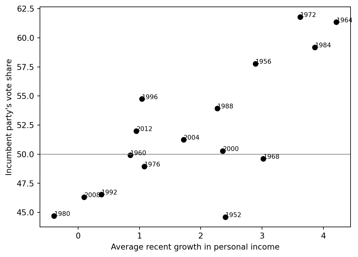
Scatter plot
Code
fig, ax = plt.subplots()ax.scatter(hibbs["growth"], hibbs["vote"], color="black")for _, r in hibbs.iterrows(): ax.text(r["growth"], r["vote"], str(int(r["year"])), fontsize=8)ax.axhline(50, color="gray", linewidth=0.8)ax.set_xlabel("Average recent growth in personal income")ax.set_ylabel("Incumbent party's vote share")
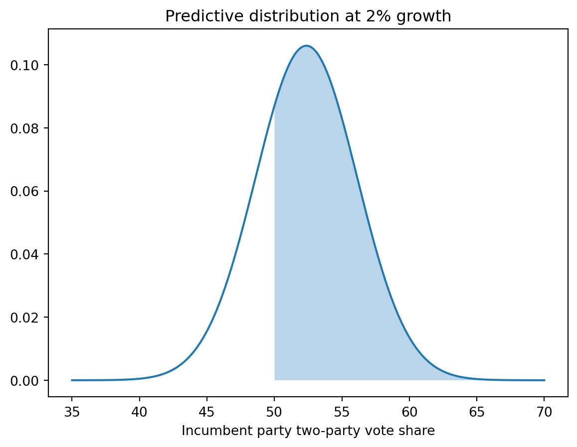
grid = np.linspace(35, 70, 500)plt.plot(grid, norm.pdf(grid, pred_mean, pred_sd))plt.fill_between(grid[grid >=50], norm.pdf(grid[grid >=50], pred_mean, pred_sd), alpha=0.3)plt.xlabel("Incumbent party two-party vote share")plt.title("Predictive distribution at 2% growth")
Text(0.5, 1.0, 'Predictive distribution at 2% growth')
CmdStanPy and BlackJAX notes
CmdStanPy gives the closest replacement for rstanarm::stan_glm if exact posterior draws are needed.
BlackJAX can sample the same Gaussian regression posterior from an explicit log density, but that adds plumbing without much pedagogical gain for this simple example.
Source Code
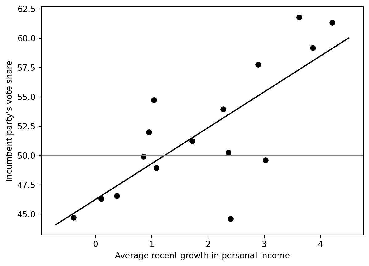
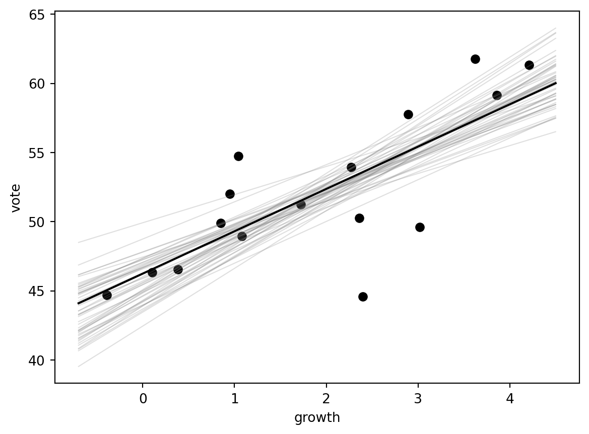
# Elections and economy: Hibbs bread-and-peace modelSource: `ElectionsEconomy/hibbs.Rmd`This ports the core linear regression and predictive simulation to Python.## Load data```{python}from pathlib import Pathimport numpy as npimport pandas as pdimport matplotlib.pyplot as pltimport statsmodels.formula.api as smffrom scipy.stats import normroot = Path("../../ROS-Examples")hibbs = pd.read_table(root /"ElectionsEconomy/data/hibbs.dat", sep=r"\s+")hibbs.head()```## Scatter plot```{python}fig, ax = plt.subplots()ax.scatter(hibbs["growth"], hibbs["vote"], color="black")for _, r in hibbs.iterrows(): ax.text(r["growth"], r["vote"], str(int(r["year"])), fontsize=8)ax.axhline(50, color="gray", linewidth=0.8)ax.set_xlabel("Average recent growth in personal income")ax.set_ylabel("Incumbent party's vote share")```## Linear regressionR original:```rM1 <-stan_glm(vote ~ growth, data = hibbs)```Python classical fit:```{python}M1 = smf.ols("vote ~ growth", data=hibbs).fit()M1.summary()``````{python}fig, ax = plt.subplots()ax.scatter(hibbs["growth"], hibbs["vote"], color="black")xs = np.linspace(-0.7, 4.5, 200)ax.plot(xs, M1.params["Intercept"] + M1.params["growth"] * xs, color="black")ax.axhline(50, color="gray", linewidth=0.8)ax.set_xlabel("Average recent growth in personal income")ax.set_ylabel("Incumbent party's vote share")```## Posterior-ish uncertainty from asymptotic normal approximationThis reproduces the book's informal Bayesian regression simulation logic.```{python}rng = np.random.default_rng(123)beta_draws = rng.multivariate_normal(M1.params.values, M1.cov_params().values, size=1000)``````{python}fig, ax = plt.subplots()ax.scatter(hibbs["growth"], hibbs["vote"], color="black", zorder=2)for b0, b1 in beta_draws[:50]: ax.plot(xs, b0 + b1 * xs, color="gray", alpha=0.25, linewidth=0.8)ax.plot(xs, M1.params["Intercept"] + M1.params["growth"] * xs, color="black")ax.set_xlabel("growth")ax.set_ylabel("vote")```## Prediction at 2% growth```{python}x_new =2.0pred_mean = M1.params["Intercept"] + M1.params["growth"] * x_newpred_sd = np.sqrt(M1.mse_resid)print(pred_mean, pred_sd)``````{python}grid = np.linspace(35, 70, 500)plt.plot(grid, norm.pdf(grid, pred_mean, pred_sd))plt.fill_between(grid[grid >=50], norm.pdf(grid[grid >=50], pred_mean, pred_sd), alpha=0.3)plt.xlabel("Incumbent party two-party vote share")plt.title("Predictive distribution at 2% growth")```## CmdStanPy and BlackJAX notes- CmdStanPy gives the closest replacement for `rstanarm::stan_glm` if exact posterior draws are needed.- BlackJAX can sample the same Gaussian regression posterior from an explicit log density, but that adds plumbing without much pedagogical gain for this simple example.