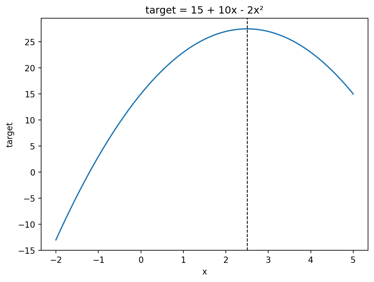
Parabola: Stan optimization in CmdStanPy and BlackJAX

Source: Parabola/parabola.Rmd

This example maximizes the unnormalized log density

\[ target(x) = 15 + 10x - 2x^2. \]

The analytic optimum is \(x = 10/4 = 2.5\).

Plot the target

Code

import numpy as np
import matplotlib.pyplot as plt

x = np.linspace(-2, 5, 400)
y = 15 + 10*x - 2*x**2
plt.plot(x, y)
plt.axvline(2.5, color="black", linestyle="--", linewidth=1)
plt.xlabel("x")
plt.ylabel("target")
plt.title("target = 15 + 10x - 2x²")

Text(0.5, 1.0, 'target = 15 + 10x - 2x²')

CmdStanPy optimization

The Stan model is identical to the original:

parameters {
  real x;
}
model {
  target += 15 + 10*x - 2*x^2;
}

Code

from pathlib import Path
from cmdstanpy import CmdStanModel

stan_file = Path("../../ROS-Examples/Parabola/parabola.stan").resolve()
model = CmdStanModel(stan_file=stan_file)
opt = model.optimize()
print(opt.optimized_params_dict)

OrderedDict({'lp__': np.float64(27.5), 'x': np.float64(2.5)})

Log-density view

For this toy example, differentiating the target is more direct than MCMC.

Code

def logdensity(x):
    return 15 + 10*x - 2*x**2

def grad_logdensity(x):
    return 10 - 4*x

x0 = 0.0
print(float(grad_logdensity(x0)))       # positive: move right
print(float(grad_logdensity(2.5)))      # zero at optimum

10.0
0.0

If we sample with NUTS, the implied normalized density is Gaussian:

\[ 15 + 10x - 2x^2 = 27.5 - 2(x - 2.5)^2, \]

so \(x \sim N(2.5, 1/4)\) after normalization.