Golf putting accuracy

Source: Golf/golf.Rmd

The data are grouped binomial counts. The logistic regression below uses lapylace.stan_glm with a binomial family and trial counts, followed by the geometry-based likelihood from the book.

Setup

from pathlib import Path
import numpy as np
import pandas as pd
import matplotlib.pyplot as plt
import lapylace as lp

root = Path("../../ROS-Examples")

def coef_medians(fit):
    return pd.Series(
        [np.median(fit.alpha_draws()), *np.median(fit.beta_draws(), axis=0)],
        index=["Intercept", *fit.columns],
    )

def fit_glm(formula, data, family=None, seed=1, prior_scale=2.5, intercept_scale=5, aux_scale=10, **kwargs):
    return lp.stan_glm(
        formula,
        data=data,
        family=family or lp.gaussian(),
        prior=lp.normal(0, prior_scale),
        prior_intercept=lp.normal(0, intercept_scale),
        prior_aux=lp.exponential(aux_scale),
        chains=2,
        parallel_chains=2,
        iter_warmup=300,
        iter_sampling=500,
        seed=seed,
        refresh=100,
        **kwargs,
    )

from scipy.special import expit
from scipy.stats import norm, binom
from scipy.optimize import minimize_scalar

golf = pd.read_csv(root / "Golf/data/golf.txt", sep=r"\s+", skiprows=2)
golf["p_hat"] = golf["y"] / golf["n"]
golf["se"] = np.sqrt(golf["p_hat"] * (1 - golf["p_hat"]) / golf["n"])
r = (1.68 / 2) / 12
R = (4.25 / 2) / 12
golf.head()

	x	n	y	p_hat	se
0	2	1443	1346	0.932779	0.006592
1	3	694	577	0.831412	0.014212
2	4	455	337	0.740659	0.020547
3	5	353	208	0.589235	0.026185
4	6	272	149	0.547794	0.030178

fit_logit = fit_glm("y ~ x", golf, family=lp.binomial(), seed=18601, prior_scale=2.5, intercept_scale=5, trials="n")
coef = coef_medians(fit_logit)
fit_logit.summary(["alpha", "beta"])

	Mean	MCSE	StdDev	5%	50%	95%	N_Eff	N_Eff/s	R_hat
alpha	2.235940	0.004140	0.061303	2.141130	2.236560	2.336880	219.294	10442.6	1.00897
beta[1]	-0.256069	0.000439	0.006606	-0.267045	-0.256062	-0.245914	226.716	10796.0	1.00431

x_grid = np.linspace(0, 1.1 * golf.x.max(), 300)
grid = pd.DataFrame({"x": x_grid, "n": 1})
p_logit = fit_logit.posterior_epred(grid).mean(axis=0)
fig, ax = plt.subplots(figsize=(7,5))
ax.errorbar(golf.x, golf.p_hat, yerr=golf.se, fmt="o", color="black", lw=.8)
ax.plot(x_grid, p_logit, color="black")
ax.set(xlabel="Distance from hole (feet)", ylabel="Probability of success", ylim=(0,1.02))

[Text(0.5, 0, 'Distance from hole (feet)'),
 Text(0, 0.5, 'Probability of success'),
 (0.0, 1.02)]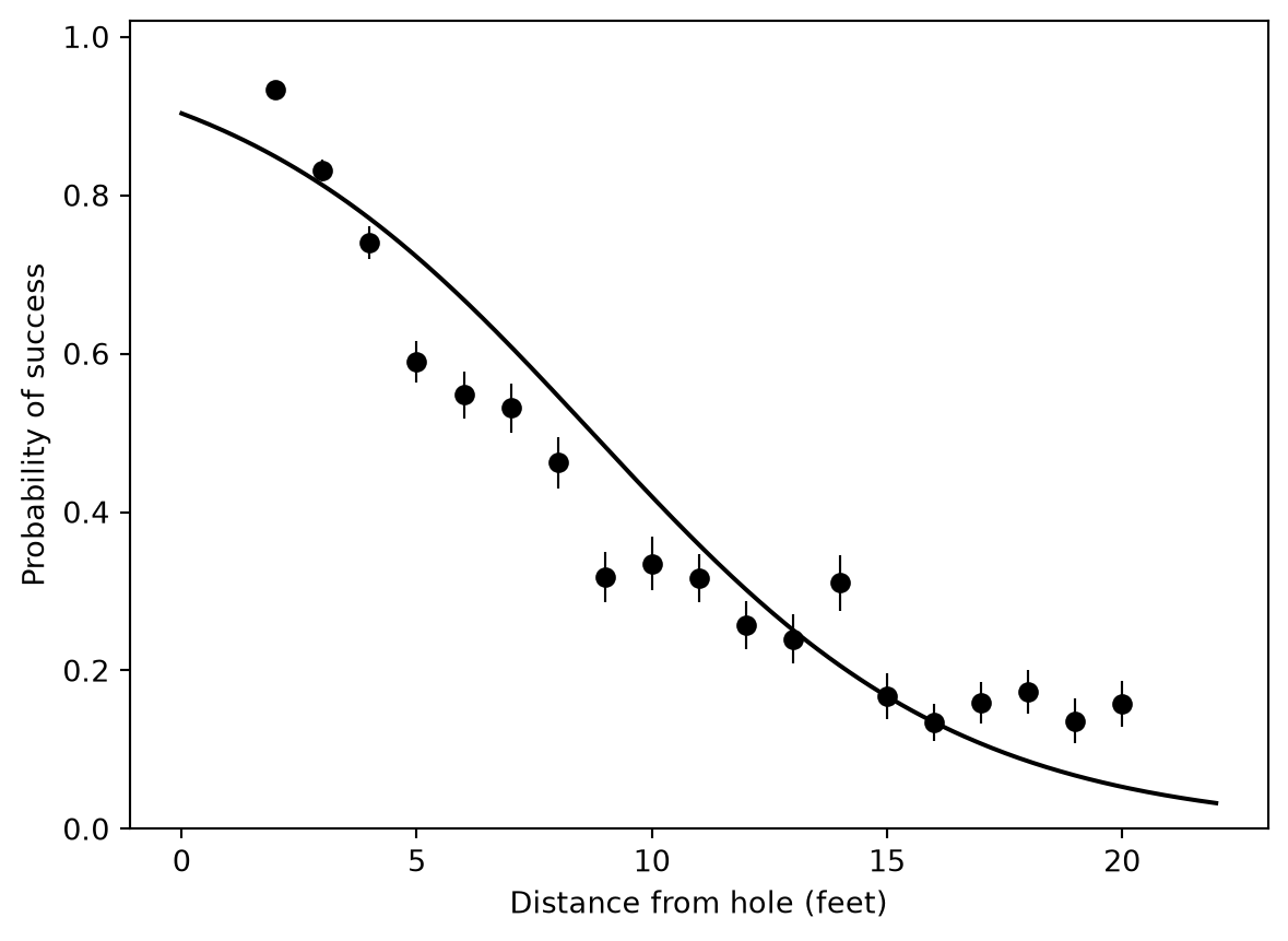

def p_geometry(x, sigma):
    x = np.asarray(x)
    p = np.ones_like(x, dtype=float)
    ok = x > (R - r)
    p[ok] = 2 * norm.cdf(np.arcsin((R - r) / x[ok]) / sigma) - 1
    return np.clip(p, 1e-9, 1 - 1e-9)

def neg_loglik(log_sigma):
    sigma = np.exp(log_sigma)
    p = p_geometry(golf.x.to_numpy(), sigma)
    return -binom.logpmf(golf.y.to_numpy(), golf.n.to_numpy(), p).sum()

opt = minimize_scalar(neg_loglik, bounds=(-6, 1), method="bounded")
sigma_hat = np.exp(opt.x)
sigma_hat, sigma_hat * 180 / np.pi

(np.float64(0.026645440807141815), np.float64(1.5266713015148838))