Staggered Adoption Panel Event Study

A reproducible panel with known dynamic treatment effects

This simulation compares matrix-panel counterfactual estimators with two PyFixest event-study specifications. It replaces the earlier vignette that required a private Hainmueller–Hangartner CSV. The results below are synthetic, not estimates from that empirical study.

Every crabbymetrics panel estimator receives fit(Y, W): a units-by-periods outcome matrix and a same-shaped, absorbing binary treatment matrix.

Data-generating process

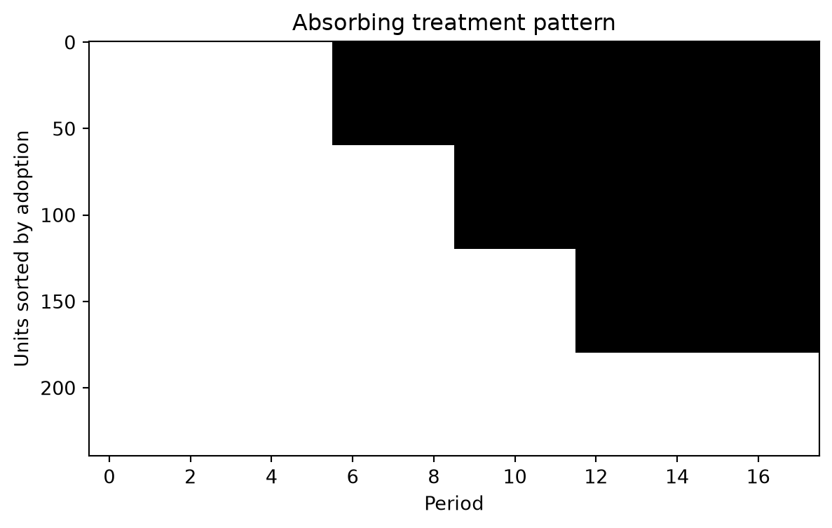
There are 240 units and 18 periods. Three cohorts adopt in periods 6, 9, and 12; the remaining units are never treated. Untreated outcomes contain unit effects, common time effects, and independent noise. Treatment effects vary with cohort and grow with exposure, so a single constant-effect TWFE coefficient is not automatically the relevant dynamic effect.

import re
import numpy as np
import pandas as pd
import matplotlib.pyplot as plt
import pyfixest as pf
import crabbymetrics as cm

rng = np.random.default_rng(20260909)
n_units, n_periods = 240, 18
periods = np.arange(n_periods)
adoption = rng.permutation(np.repeat([6, 9, 12, 999], n_units // 4))
relative = periods[None, :] - adoption[:, None]
W = (relative >= 0).astype(float)
unit_effect = rng.normal(size=(n_units, 1))
time_effect = 0.04 * periods + 0.2 * np.sin(periods / 3)
untreated = unit_effect + time_effect + rng.normal(scale=0.35, size=W.shape)
cohort_shift = np.where(adoption == 999, 0.0, 0.1 * (adoption - 6) / 3)
true_effect = W * (0.8 + cohort_shift[:, None] + 0.12 * np.maximum(relative, 0))
Y = untreated + true_effect
true_att = float(true_effect[W == 1].mean())

df = pd.DataFrame({
    "unit": np.repeat(np.arange(n_units), n_periods),
    "period": np.tile(periods, n_units),
    "outcome": Y.ravel(),
    "g": np.repeat(np.where(adoption == 999, 0, adoption), n_periods),
    "treated": W.ravel(),
    "truth": true_effect.ravel(),
})
print("Y and W shapes:", Y.shape, W.shape)
print("True treated-cell average:", round(true_att, 3))

Y and W shapes: (240, 18) (240, 18)
True treated-cell average: 1.398

fig, ax = plt.subplots(figsize=(7, 4))
ax.imshow(W[np.argsort(adoption)], aspect="auto", interpolation="nearest", cmap="Greys")
ax.set(xlabel="Period", ylabel="Units sorted by adoption", title="Absorbing treatment pattern")
plt.show()

Matrix-panel estimators

HorizontalPanelRidge, MatrixCompletion, and SyntheticDID provide scalar effects and nested event-study summaries. Always inspect convergence diagnostics where available. MatrixCompletion can retain a nonconverged iterate on budget exhaustion; returning from fit alone is not a convergence check.

estimators = {
    "HorizontalPanelRidge": cm.HorizontalPanelRidge(1.0),
    "MatrixCompletion": cm.MatrixCompletion(max_iterations=1000, tolerance=1e-5),
    "SyntheticDID": cm.SyntheticDID(),
}
paths = {}
rows = []
for name, estimator in estimators.items():
    estimator.fit(Y, W)
    result = (estimator.summary(include_matrices=False)
              if name == "MatrixCompletion" else estimator.summary())
    event = result["event_study"]["weighted"]
    paths[name] = pd.DataFrame({
        "event_time": event["event_time"],
        "estimate": event["estimate"],
        "n": event["n"],
    })
    rows.append({
        "estimator": name,
        "att": result["att"],
        "converged": result.get("converged", "not reported"),
    })
display(pd.DataFrame(rows))
assert all(row["converged"] != False for row in rows)

	estimator	att	converged
0	HorizontalPanelRidge	1.455108	not reported
1	MatrixCompletion	1.393187	True
2	SyntheticDID	1.407768	True

These scalar outputs do not necessarily use the same weighting as the raw treated-cell average. SyntheticDID’s scalar ATT uses both unit and time weights; its event path is a period-specific weighted gap. Counterfactual-model assumptions and cohort weights matter even when every method accepts the same matrices.

Two-way fixed effects and saturated event studies

The first PyFixest fit pools event-time effects across cohorts. The second fits cohort-specific effects and aggregates them using the saturated/Sun-Abraham-style interface. Both use unit-clustered intervals and period -1 as the reference. The outermost TWFE event times are binned.

df["rel"] = np.where(df.g > 0, df.period - df.g, -999)
df["rel_bin"] = df.rel.clip(-5, 5).astype(int).astype(str)
df.loc[df.g == 0, "rel_bin"] = "never"
twfe = pf.feols(
    'outcome ~ i(rel_bin, ref="-1") | unit + period',
    data=df, vcov={"CRV1": "unit"},
)
tidy = twfe.tidy().reset_index().rename(columns={"Coefficient": "term"})
twfe_rows = []
for _, row in tidy.iterrows():
    match = re.search(r"rel_bin::(-?\d+)", str(row["term"]))
    if match:
        twfe_rows.append({
            "event_time": int(match.group(1)),
            "estimate": row["Estimate"],
            "lower": row["2.5%"],
            "upper": row["97.5%"],
        })
twfe_event = pd.DataFrame(twfe_rows).sort_values("event_time")
assert len(twfe_event) > 1

saturated = pf.event_study(
    df, yname="outcome", idname="unit", tname="period", gname="g",
    estimator="saturated", att=False, cluster="unit",
)
sa_event = saturated.aggregate().reset_index().rename(columns={
    "period": "event_time", "Estimate": "estimate",
    "2.5%": "lower", "97.5%": "upper",
})
display(sa_event[["event_time", "estimate", "lower", "upper"]].head())

	event_time	estimate	lower	upper
0	-12.0	-0.065855	-0.247805	0.116094
1	-11.0	-0.22325	-0.382263	-0.064237
2	-10.0	-0.10984	-0.281875	0.062194
3	-9.0	-0.054269	-0.164751	0.056213
4	-8.0	-0.035436	-0.149147	0.078275

Event paths and known effects

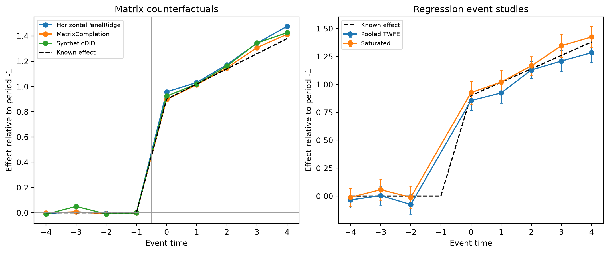
For display, matrix-estimator paths are centered on their own period -1 estimate. This makes their normalization explicit; it does not make their weighting identical to PyFixest’s. The truth curve averages effects among the ever-treated units observed at each event time. Restricting to interior periods avoids interpreting the binned TWFE endpoints as single-period effects.

truth = df.loc[df.g > 0].groupby("rel").truth.mean()
fig, axes = plt.subplots(1, 2, figsize=(11, 4.5), constrained_layout=True)
for name, path in paths.items():
    baseline = path.loc[path.event_time.eq(-1), "estimate"].iloc[0]
    shown = path.loc[path.event_time.between(-4, 4)]
    axes[0].plot(shown.event_time, shown.estimate - baseline, marker="o", label=name)
for label, path in [("Pooled TWFE", twfe_event), ("Saturated", sa_event)]:
    shown = path.loc[path.event_time.between(-4, 4)]
    axes[1].errorbar(
        shown.event_time, shown.estimate,
        yerr=np.vstack([shown.estimate - shown.lower, shown.upper - shown.estimate]),
        marker="o", capsize=2, label=label,
    )
for ax, title in zip(axes, ["Matrix counterfactuals", "Regression event studies"]):
    shown_truth = truth.loc[(truth.index >= -4) & (truth.index <= 4)]
    ax.plot(shown_truth.index, shown_truth, color="black", linestyle="--", label="Known effect")
    ax.axhline(0, color="0.6", linewidth=0.7)
    ax.axvline(-0.5, color="0.6", linewidth=0.7)
    ax.set(xlabel="Event time", ylabel="Effect relative to period -1", title=title)
    ax.legend(fontsize=8)
plt.show()

A single simulated sample is not a coverage study. The matrix curves are point estimates without event-time confidence bands; the regression intervals reflect their own clustered covariance assumptions. Use the panel DGP Monte Carlo for repeated-sample comparisons, and the real panel case studies for empirical examples with bundled data.