Estimator scaling and reference implementations

Fresh v0.9.0 timings for the 30-estimator benchmark inventory

This ablation reruns the 30-estimator benchmark inventory against v0.9.0, using adapter revision 2. The bounded grid is \(n \in \{10^3,10^4,10^5\}\) and \(k \in \{5,20\}\). It does not include the newly added MPE_CBPS, which has its own executed API example and Chronos simulation.

The September 9 measurements replace the obsolete August charts. They include the corrected unpenalized GLM, centered ElasticNet, same-panel horizontal ridge, same-sample 2SLS, and R fit-only timing adapters. This is a smaller reproducible profiling grid, not a rerun of the old \(10^7\)-row sweep.

The benchmark README documents reference implementations and dimension conventions. Download the measurements and host metadata.

Guard rails

Each cell runs in a fresh subprocess with single-threaded numerical kernels. The driver rejects predicted over-cap allocations, watches aggregate descendant RSS, enforces a wall timeout, and stops attempting larger samples after the first hard failure for an estimator/implementation/dimension path. Thus a missing point is an observed feasibility boundary, not an accidental omission.

Code
from pathlib import Path
import sys
import json

import matplotlib.pyplot as plt
import numpy as np
import pandas as pd
from IPython.display import Markdown, display

path = Path("data/estimator-scaling.csv")
results = pd.read_csv(path)
host = json.loads(path.with_suffix(".host.json").read_text())
assert set(results.adapter_revision.dropna()) == {2}
assert set(results.loc[results.implementation.eq("crabbymetrics") & results.status.eq("ok"), "library_version"]) == {"0.9.0"}

benchmark_root = Path.cwd().parents[1] / "benchmarks" / "scaling"
sys.path.insert(0, str(benchmark_root))
from registry import ESTIMATORS, REFERENCE_URLS
from report_metadata import EXPERIMENT_DETAILS


def scaling_slope(frame):
    frame = frame.loc[
        frame.status.eq("ok")
        & frame.fit_seconds.gt(0)
        & frame.n.gt(0)
    ].drop_duplicates("n")
    if len(frame) < 3:
        return np.nan
    return np.polyfit(np.log10(frame.n), np.log10(frame.fit_seconds), deg=1)[0]


def render_estimator(estimator):
    detail = EXPERIMENT_DETAILS[estimator]
    spec = ESTIMATORS[estimator]
    references = []
    for reference in spec["references"]:
        url = REFERENCE_URLS[reference]
        if url.startswith("../../"):
            url = "https://github.com/apoorvalal/crabbymetrics/blob/v0.9.0/" + url[6:]
        references.append(f"[{reference}]({url})" if url else reference)
    display(
        Markdown(
            f"**Family and dimensions.** `{spec['family']}`; `k` means "
            f"{spec['k_semantics']}.\n\n"
            f"**Data-generating process.** {detail['dgp']}\n\n"
            f"**Fitted specification.** {detail['fit']}\n\n"
            f"**Reference interpretation.** {detail['comparison']}\n\n"
            f"**Reference code.** {', '.join(references)}"
        )
    )

    frame = results.loc[results.estimator.eq(estimator)].copy()
    ok = frame.loc[frame.status.eq("ok")].copy()
    frontier = (
        ok.groupby("implementation", dropna=False)
        .agg(
            max_completed_n=("n", "max"),
            max_completed_k=("k", "max"),
            median_fit_seconds=("fit_seconds", "median"),
            max_peak_rss_gib=("peak_rss_bytes", lambda values: values.max() / 2**30),
        )
        .reset_index()
    )
    summary = (
        frame.groupby("implementation", dropna=False)
        .agg(
            completed=("status", lambda values: int((values == "ok").sum())),
            timeouts=("status", lambda values: int((values == "timeout").sum())),
            rss_kills=("status", lambda values: int((values == "killed_rss_guard").sum())),
            preflight_skips=("status", lambda values: int((values == "preflight_oom").sum())),
        )
        .reset_index()
        .merge(frontier, how="left", on="implementation")
    )
    slopes = (
        frame.groupby(["implementation", "k"], dropna=False)
        .apply(scaling_slope, include_groups=False)
        .dropna()
        .groupby("implementation")
        .agg(median_log_log_slope="median", slope_paths="size")
        .reset_index()
    )
    summary = summary.merge(slopes, how="left", on="implementation")
    summary["max_completed_n"] = summary.max_completed_n.fillna(0).astype(int)
    summary["max_completed_k"] = summary.max_completed_k.fillna(0).astype(int)
    display(
        summary.rename(
            columns={
                "implementation": "implementation",
                "completed": "completed cells",
                "timeouts": "timeouts",
                "rss_kills": "RSS kills",
                "preflight_skips": "preflight skips",
                "max_completed_n": "largest completed n",
                "max_completed_k": "largest completed k",
                "median_fit_seconds": "median fit seconds",
                "max_peak_rss_gib": "maximum observed RSS (GiB)",
                "median_log_log_slope": "median log-log runtime slope",
                "slope_paths": "k paths with slope",
            }
        )
    )

    if ok.empty:
        return
    fig, axes = plt.subplots(1, 2, figsize=(11, 4.2))
    for (implementation, k), group in ok.groupby(["implementation", "k"]):
        group = group.sort_values("n")
        label = f"{implementation}, k={int(k)}"
        axes[0].plot(group.n, group.fit_seconds, marker="o", linewidth=1, label=label)
        axes[1].plot(
            group.n,
            group.peak_rss_bytes / 2**30,
            marker="o",
            linewidth=1,
            label=label,
        )
    axes[0].set(xscale="log", yscale="log", xlabel="n", ylabel="fit seconds")
    axes[1].set(xscale="log", yscale="log", xlabel="n", ylabel="peak child RSS (GiB)")
    axes[0].set_title("Runtime scaling")
    axes[1].set_title("Memory scaling")
    handles, labels = axes[0].get_legend_handles_labels()
    fig.legend(handles, labels, loc="outside lower center", ncol=3, fontsize=6)
    fig.suptitle(estimator)
    fig.tight_layout(rect=(0, 0.16, 1, 1))
    plt.show()

Completion status

The status table includes every requested cell. Timeouts and pruned larger cells are retained as feasibility outcomes; successful timings alone do not describe the whole grid.

Code
print("Cells:", len(results))
print("Native estimator inventory:", results.loc[results.implementation.eq("crabbymetrics"), "estimator"].nunique())
print("Generated at:", host["generated_at_utc"])
print("Platform:", host["platform"])
print("Effective RSS cap (GiB):", round(host["memory_cap_bytes"] / 2**30, 2))
print("Per-cell timeout (s):", host["arguments"]["timeout"])
if results.empty:
    print("Run benchmarks/scaling/run_grid.py to populate the guarded grid.")
else:
    display(
        results.groupby(["implementation", "status"], dropna=False)
        .size()
        .rename("cells")
        .reset_index()
        .sort_values(["implementation", "status"])
    )
Cells: 276
Native estimator inventory: 30
Generated at: 2026-09-09T15:25:05.241640+00:00
Platform: macOS-26.6.2-arm64-arm-64bit
Effective RSS cap (GiB): 1.32
Per-cell timeout (s): 10.0
implementation status cells
0 crabbymetrics ok 168
1 crabbymetrics pruned_after_failure 5
2 crabbymetrics timeout 7
3 doubleml-irm ok 6
4 doubleml-plr ok 6
5 lifelines-cox-ph ok 6
6 pyfixest-feols ok 6
7 pyfixest-iv ok 6
8 r-fixest-feols ok 6
9 r-survival-andersen-gill ok 6
10 r-survival-coxph ok 6
11 sklearn-bagged-polynomial ok 6
12 sklearn-elastic-net ok 6
13 sklearn-linear-regression ok 6
14 sklearn-logistic-regression ok 6
15 sklearn-multinomial-logit ok 6
16 sklearn-poisson-regressor ok 6
17 sklearn-ridge ok 12

Numerical experiment

Common grid and timing boundary

This run is the Cartesian product of three sample sizes and two dimensions. A fresh seeded generator builds the complete input outside the fit timer. The reported fit_seconds starts immediately before the estimator call and stops on return; imports and data generation are excluded. In contrast, peak_rss_bytes covers the complete child process, including imported libraries, generated inputs, copies made by foreign-function boundaries, solver workspaces, and descendants such as R subprocesses.

The preflight starts from the raw \(8nk\) bytes for a float64 design (or the family-specific panel/dynamic analogue), multiplies it by a conservative estimator-family workspace factor, and adds 192 MiB. The run-time monitor then enforces the requested 2 GiB cap or available RAM after a 4 GiB system reserve, whichever is smaller. The effective cap is printed above. Every child and descendant is subject to a 10-second wall clock. A preflight rejection, RSS kill, timeout, or execution error stops larger n values only for that estimator, implementation, and k path.

Dimension conventions

  • Tabular, GLM, IV, survival, moment, balancing, and semiparametric estimators: n rows and k covariates/instruments.
  • Synthetic control: n pre-treatment periods and k donor series.
  • Other panel estimators: n periods and k units; this is a matrix stress dimension, not an ordinary covariate count.
  • Dynamic estimators: approximately n/4 units, four decision periods, and k history covariates.

Randomness and comparability

All cells use seed 1729 and single-threaded BLAS/OpenMP/Rcpp settings. Each cell is measured once; sub-millisecond ratios are especially sensitive to noise. Native and external adapters reconstruct the same DGP and shape. The experiment measures systems scaling, not statistical accuracy. Only references with a defensible generic-grid adapter enter timing comparisons; related-but-different estimators remain linked as provenance and are explicitly described below.

Matched reference ratios

The table below uses only cells where both Crabbymetrics and the external implementation completed. reference / native > 1 means the Crabbymetrics fit was faster; values below one mean the external fit was faster. Medians summarize heterogeneous \((n,k)\) cells and should be read as a profiling signal, not a single universal speed factor.

Code
if not results.empty:
    native = (
        results.loc[
            results.implementation.eq("crabbymetrics") & results.status.eq("ok"),
            ["estimator", "n", "k", "fit_seconds"],
        ]
        .rename(columns={"fit_seconds": "native_seconds"})
    )
    matched = (
        results.loc[
            results.implementation.ne("crabbymetrics") & results.status.eq("ok")
        ]
        .merge(native, on=["estimator", "n", "k"])
        .assign(reference_over_native=lambda frame: frame.fit_seconds / frame.native_seconds)
    )
    ratios = (
        matched.groupby(["estimator", "implementation"])
        .agg(
            matched_cells=("reference_over_native", "size"),
            median_reference_over_native=("reference_over_native", "median"),
        )
        .reset_index()
    )
    display(ratios)
estimator implementation matched_cells median_reference_over_native
0 AIPW doubleml-irm 6 4.383541
1 AndersenGill r-survival-andersen-gill 3 0.019379
2 BaggedPolynomialRegressor sklearn-bagged-polynomial 5 0.315952
3 CoxPH lifelines-cox-ph 6 46.853864
4 CoxPH r-survival-coxph 6 4.001714
5 ElasticNet sklearn-elastic-net 6 3.140382
6 FixedEffectsOLS pyfixest-feols 6 6.544128
7 FixedEffectsOLS r-fixest-feols 6 5.600785
8 HorizontalPanelRidge sklearn-ridge 6 4.177901
9 Logit sklearn-logistic-regression 6 1.435108
10 MultinomialLogit sklearn-multinomial-logit 6 0.156895
11 OLS sklearn-linear-regression 6 4.281109
12 PartiallyLinearDML doubleml-plr 6 1.446912
13 Poisson sklearn-poisson-regressor 6 1.862092
14 Ridge sklearn-ridge 6 3.774888
15 TwoSLS pyfixest-iv 6 2.401204

Estimator-by-estimator results

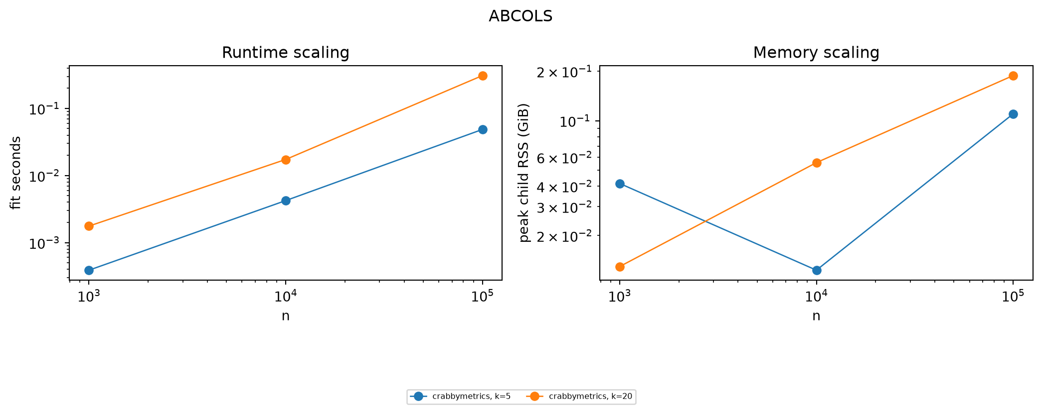
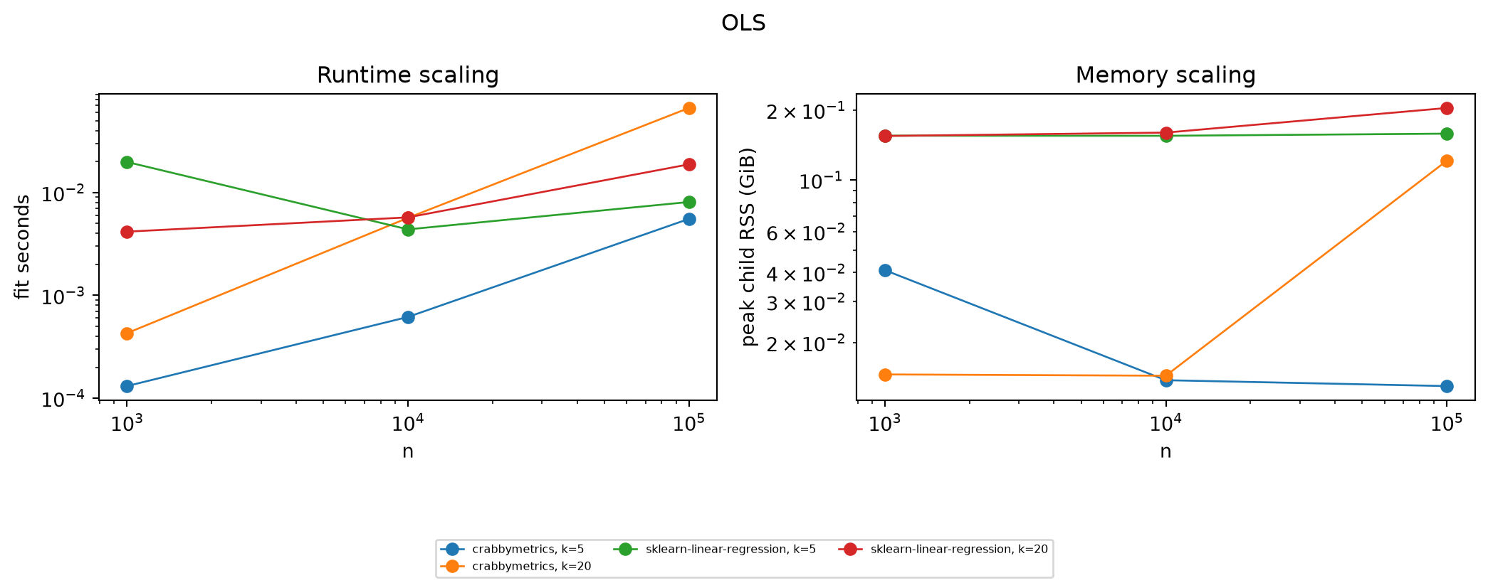
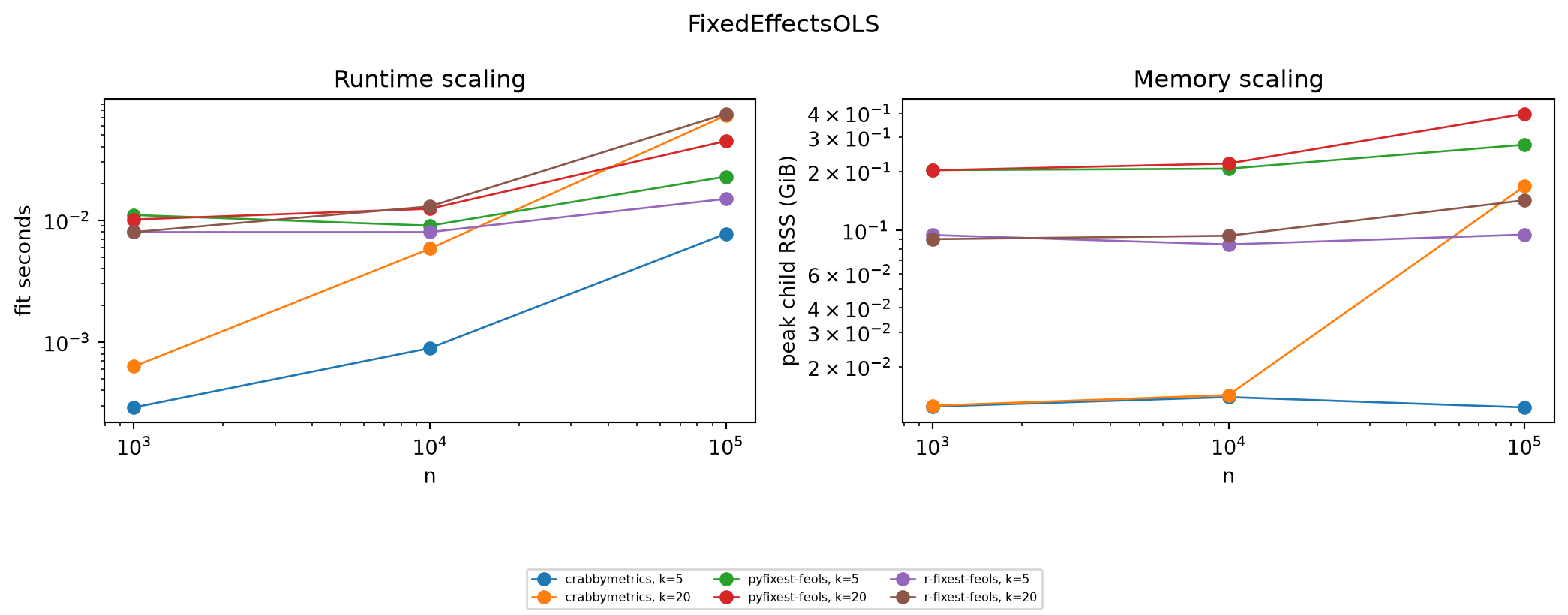
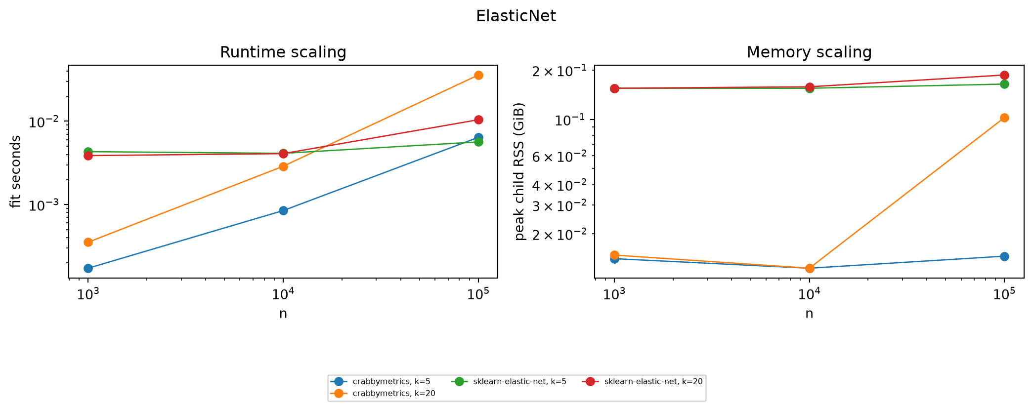
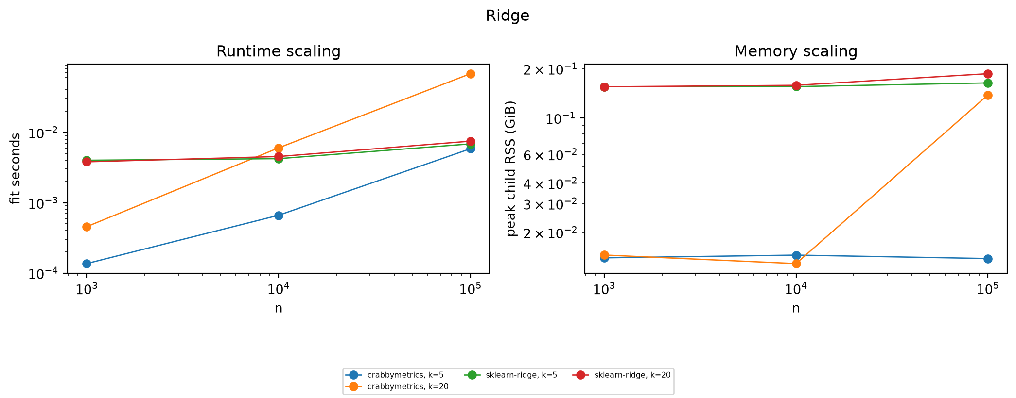
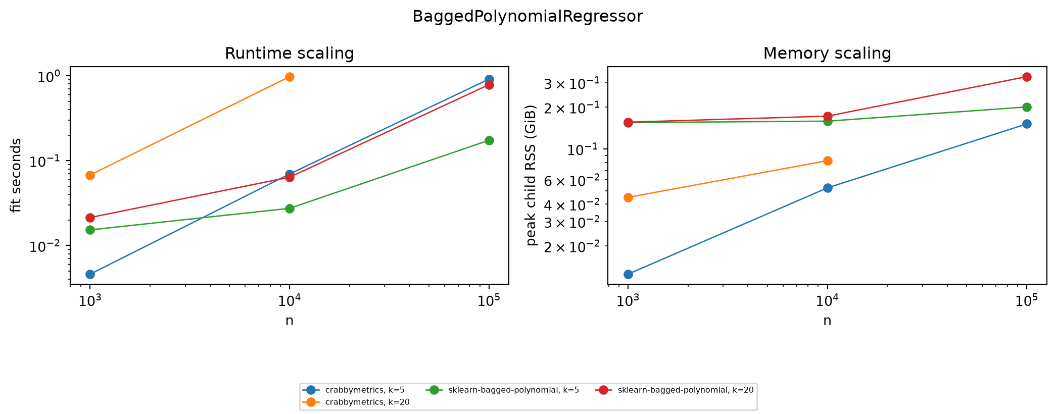
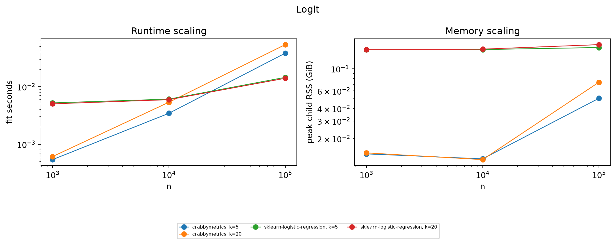
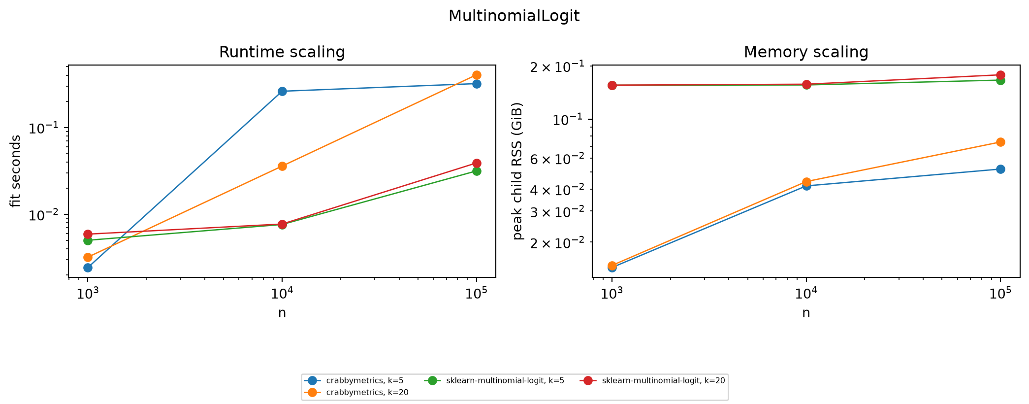
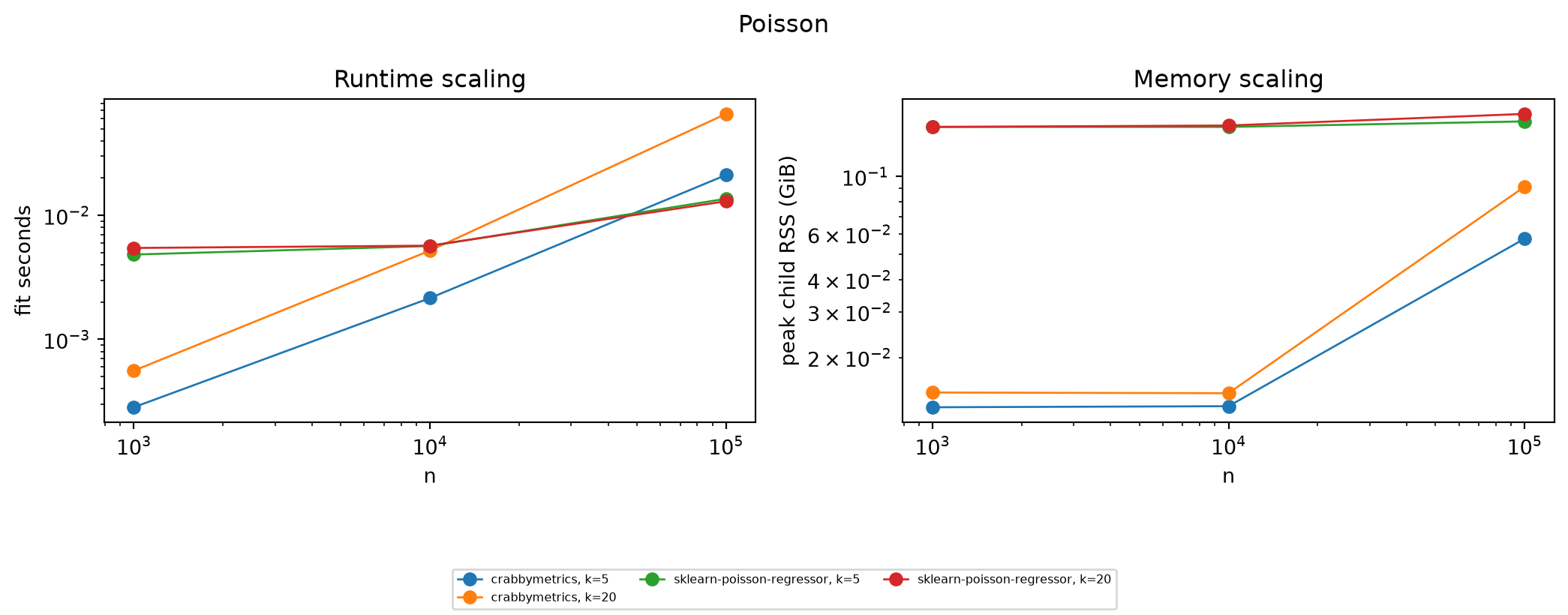
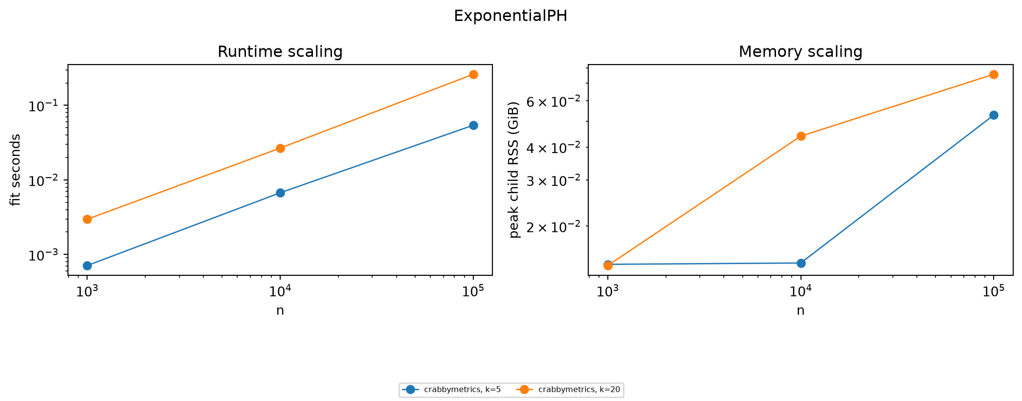
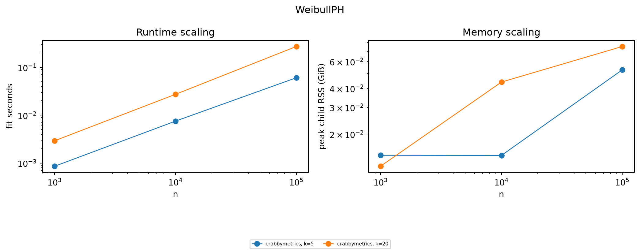
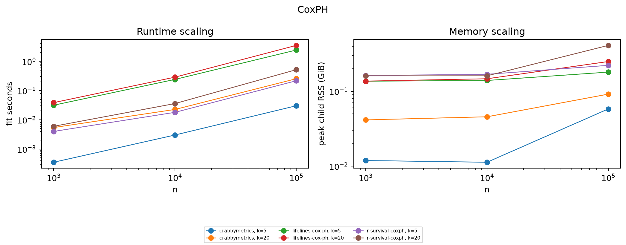
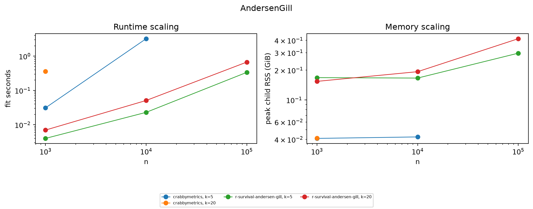
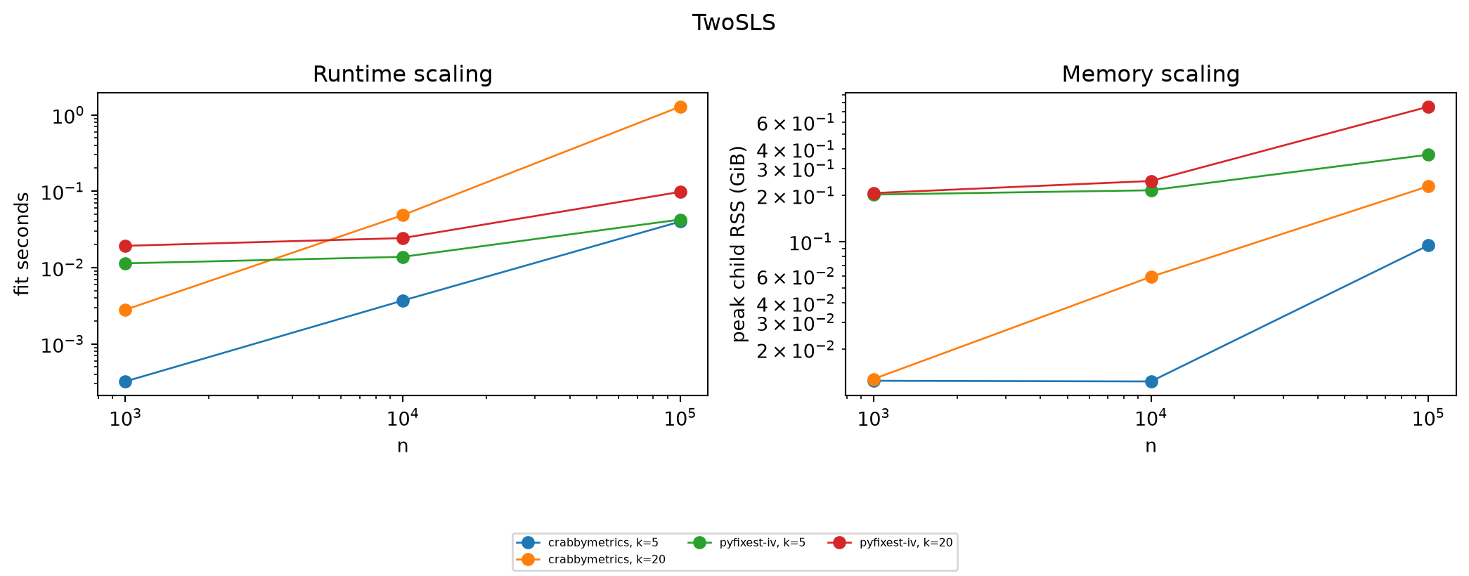
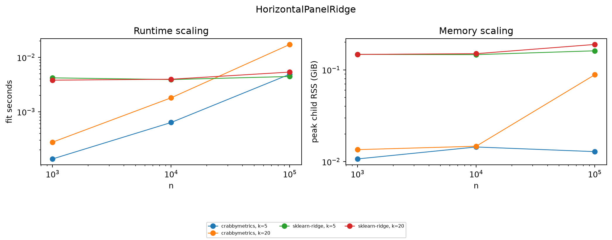
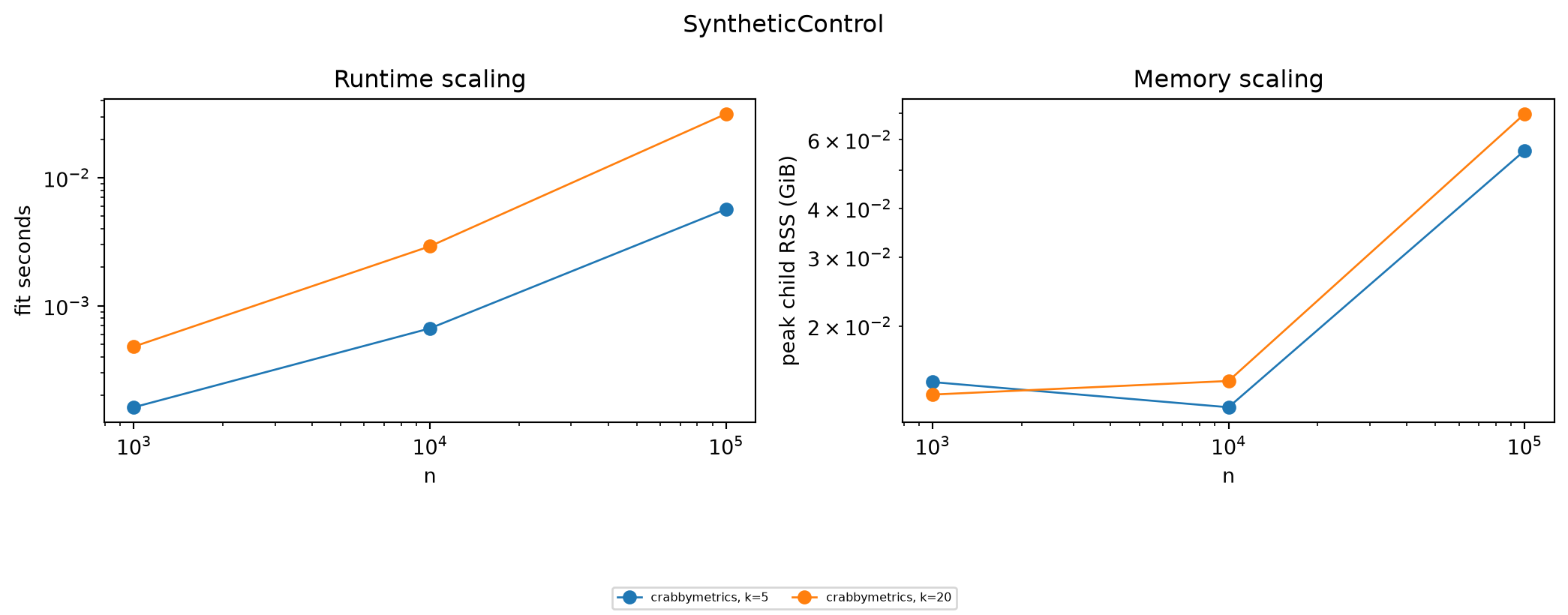
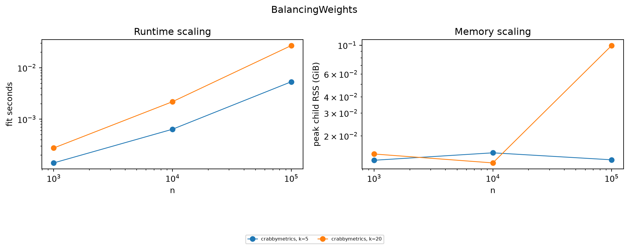
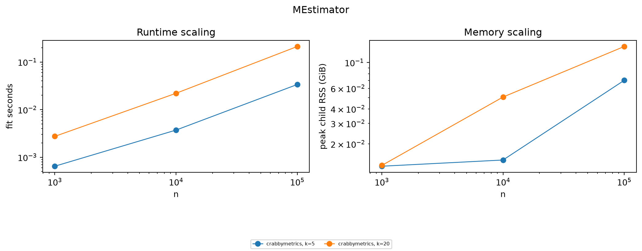
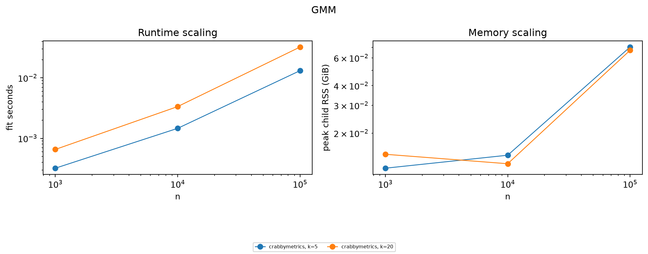
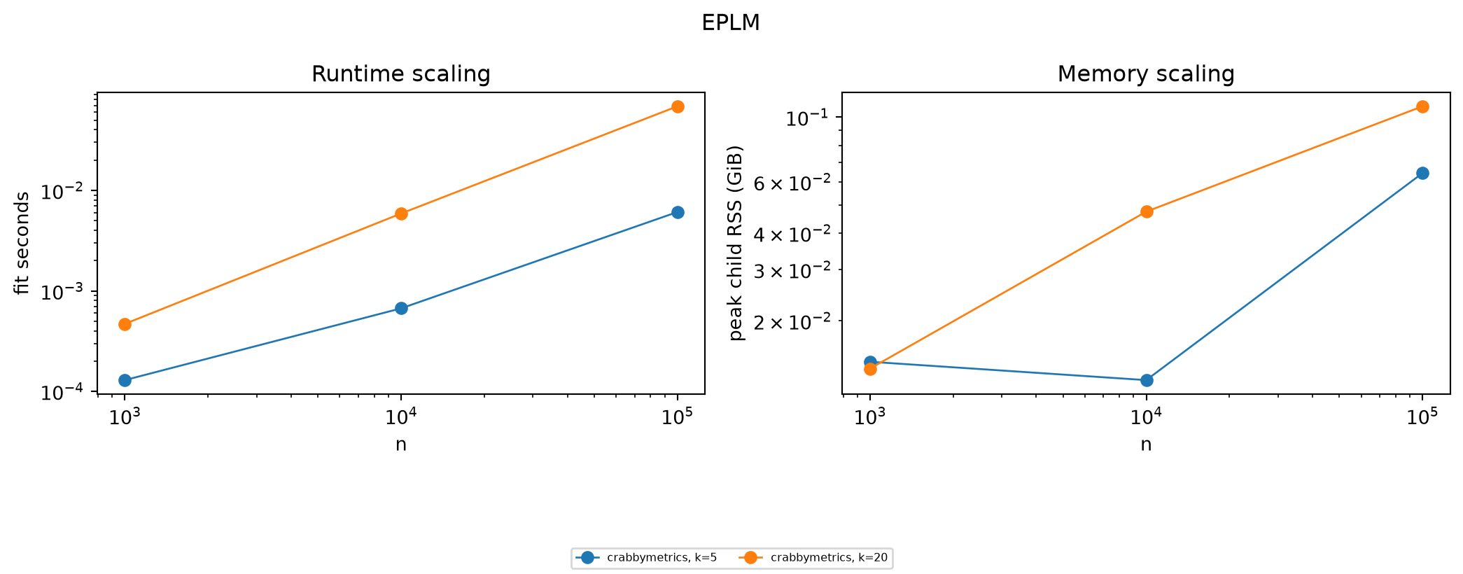
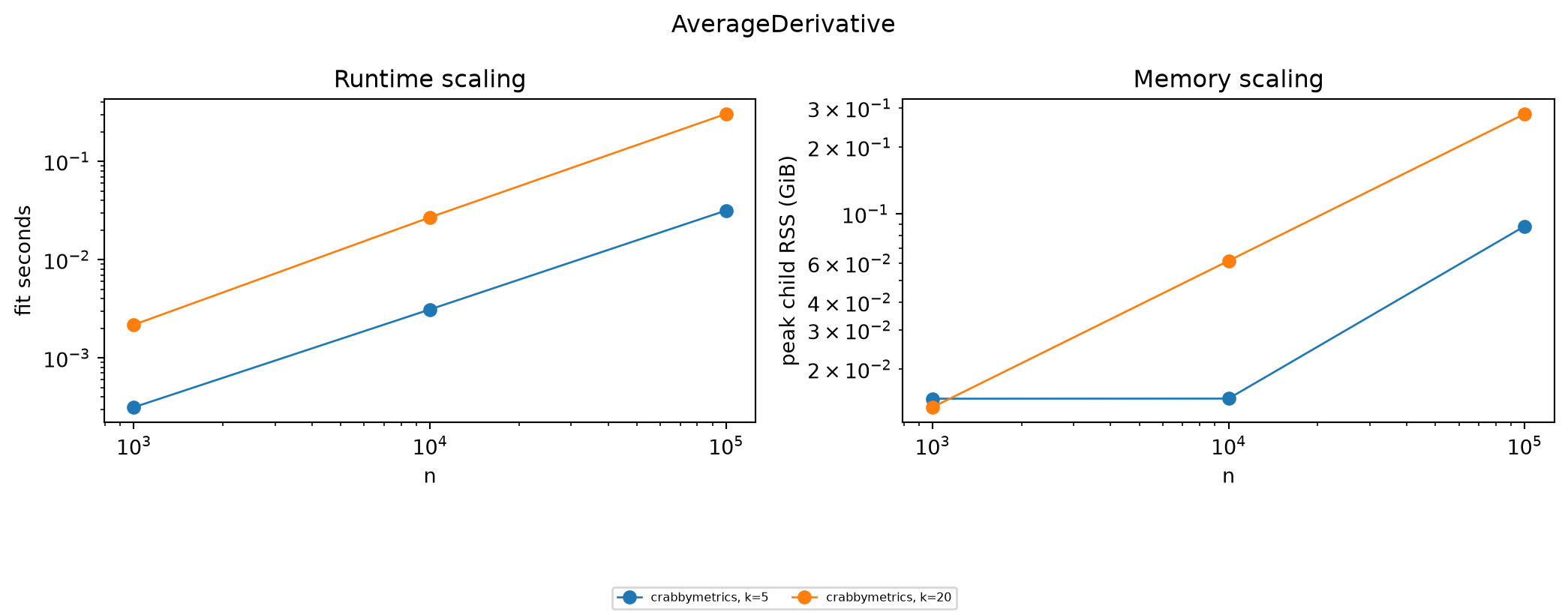
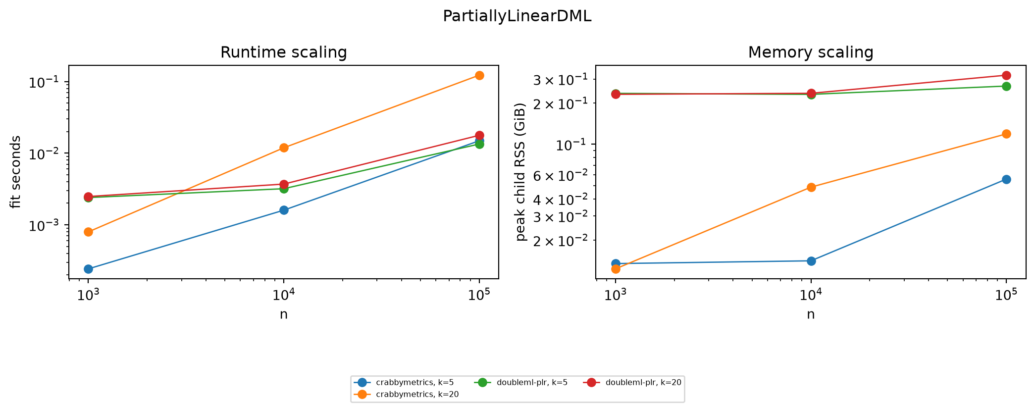
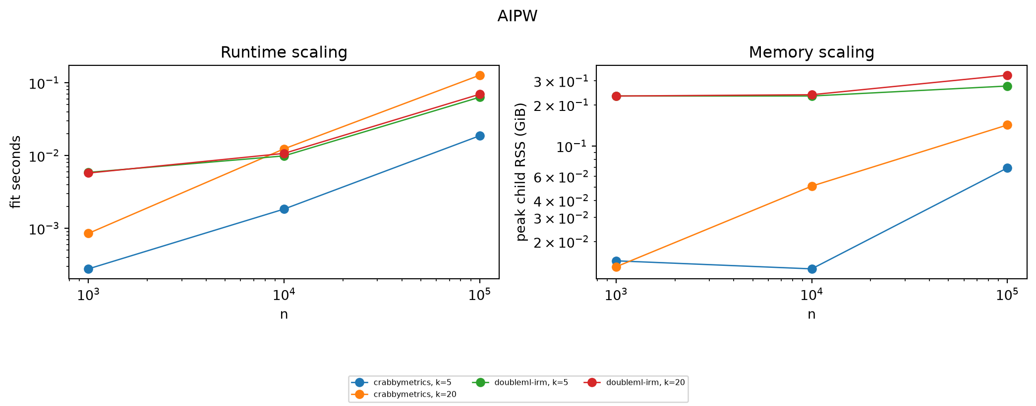
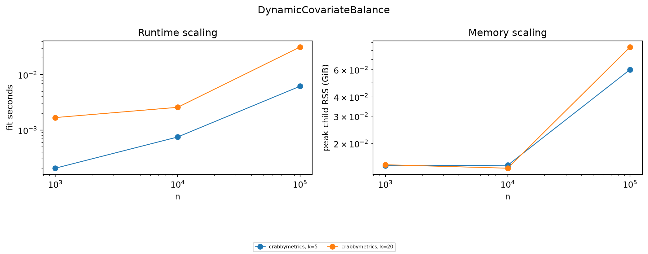
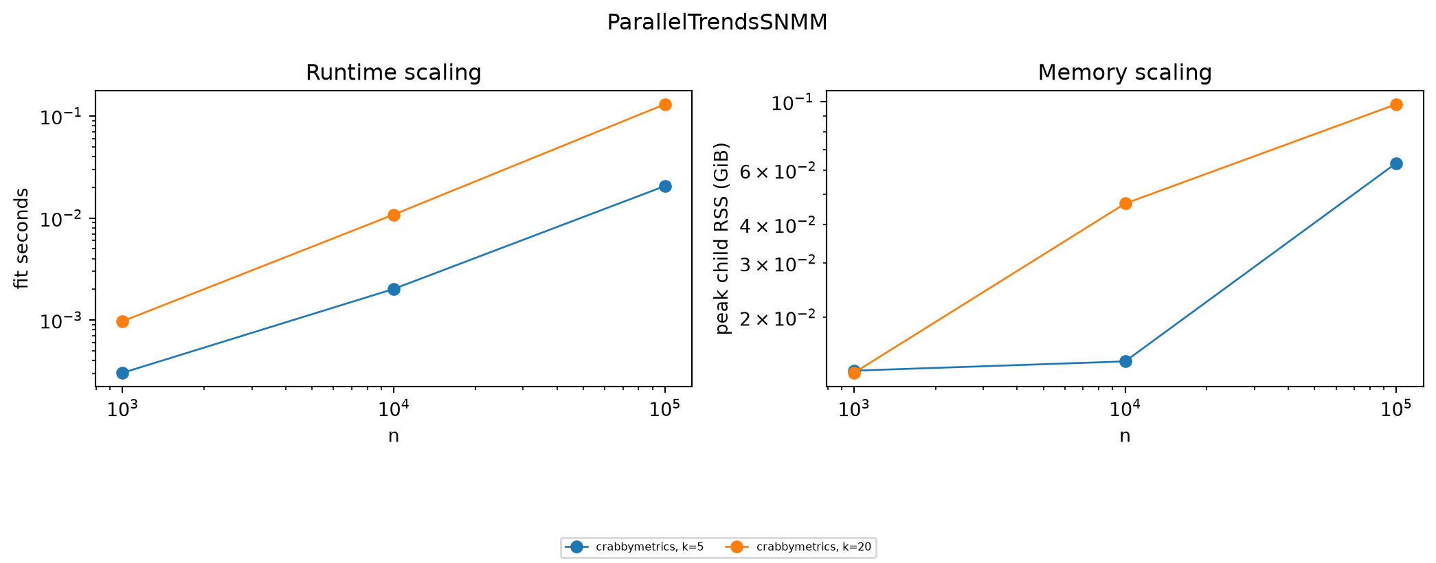
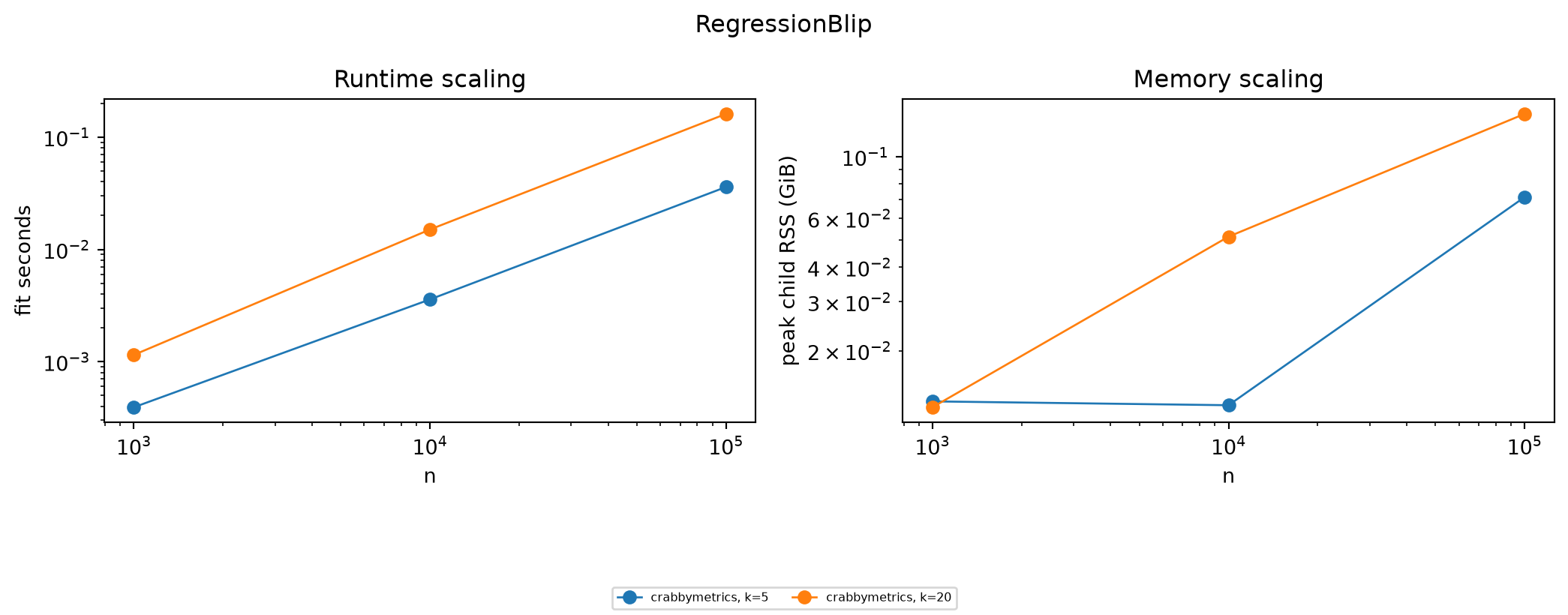
Each subsection gives the exact DGP, fitted tuning values, reference status, completion frontier, median log-log runtime slope, and two scaling plots. A log-log slope near one indicates approximately linear empirical scaling along a fixed-k path; it is descriptive and can mix solver regimes over this short grid.

ABCOLS

Family and dimensions. tabular; k means continuous covariates (plus two categorical variables).

Data-generating process. Gaussian linear outcome with n rows and k standard-normal continuous covariates; two deterministic categorical variables cycle through 8 and 5 levels.

Fitted specification. ABCOLS with centered continuous covariates and categorical main effects; the scaling run does not add continuous-by-category or category-by-category interactions.

Reference interpretation. No exact public implementation was found. R wec is retained as weighted-effect-coding provenance, not timed as an equivalent estimator.

Reference code. r-wec

implementation completed cells timeouts RSS kills preflight skips largest completed n largest completed k median fit seconds maximum observed RSS (GiB) median log-log runtime slope k paths with slope
0 crabbymetrics 6 0 0 0 100000 20 0.010777 0.188293 1.085267 2

OLS

Family and dimensions. tabular; k means covariates.

Data-generating process. Gaussian linear outcome y = X beta + epsilon with X of shape n by k, beta_j increasing from 0.2 to 1 and normalized by sqrt(k), and unit-variance noise.

Fitted specification. Unpenalized Crabbymetrics OLS versus scikit-learn LinearRegression, both with their normal intercept conventions.

Reference interpretation. Shape- and estimand-matched timing comparison.

Reference code. sklearn-linear-regression

implementation completed cells timeouts RSS kills preflight skips largest completed n largest completed k median fit seconds maximum observed RSS (GiB) median log-log runtime slope k paths with slope
0 crabbymetrics 6 0 0 0 100000 20 0.003077 0.121155 0.953773 2
1 sklearn-linear-regression 6 0 0 0 100000 20 0.006907 0.204300 0.066335 2

FixedEffectsOLS

Family and dimensions. fixed-effects; k means covariates.

Data-generating process. The Gaussian linear design plus one fixed-effect identifier cycling over min(1000, n/20) groups.

Fitted specification. Crabbymetrics within-transformed FixedEffectsOLS versus PyFixest feols and R fixest feols with iid covariance work requested.

Reference interpretation. Same outcome, covariates, and one-way fixed-effect partition; implementation overhead and covariance defaults can still differ.

Reference code. pyfixest-feols, r-fixest-feols

implementation completed cells timeouts RSS kills preflight skips largest completed n largest completed k median fit seconds maximum observed RSS (GiB) median log-log runtime slope k paths with slope
0 crabbymetrics 6 0 0 0 100000 20 0.003372 0.168350 0.872444 2
1 pyfixest-feols 6 0 0 0 100000 20 0.011740 0.396469 0.240293 2
2 r-fixest-feols 6 0 0 0 100000 20 0.010500 0.142639 0.311243 2

ElasticNet

Family and dimensions. tabular; k means covariates.

Data-generating process. The Gaussian linear design with n rows and k covariates.

Fitted specification. Penalty 0.01, l1 ratio 0.5, and at most 300 iterations in Crabbymetrics and scikit-learn.

Reference interpretation. Matched regularization family and tuning values; stopping criteria are library-specific.

Reference code. sklearn-elastic-net

implementation completed cells timeouts RSS kills preflight skips largest completed n largest completed k median fit seconds maximum observed RSS (GiB) median log-log runtime slope k paths with slope
0 crabbymetrics 6 0 0 0 100000 20 0.001864 0.102570 0.894483 2
1 sklearn-elastic-net 6 0 0 0 100000 20 0.004213 0.186844 0.136836 2

Ridge

Family and dimensions. tabular; k means covariates.

Data-generating process. The Gaussian linear design with n rows and k covariates.

Fitted specification. Unit ridge penalty in Crabbymetrics and scikit-learn.

Reference interpretation. Matched penalized least-squares problem modulo intercept and solver conventions.

Reference code. sklearn-ridge

implementation completed cells timeouts RSS kills preflight skips largest completed n largest completed k median fit seconds maximum observed RSS (GiB) median log-log runtime slope k paths with slope
0 crabbymetrics 6 0 0 0 100000 20 0.003252 0.138046 0.951604 2
1 sklearn-ridge 6 0 0 0 100000 20 0.004378 0.186264 0.131524 2

BaggedPolynomialRegressor

Family and dimensions. polynomial; k means raw covariates.

Data-generating process. The Gaussian linear design is deliberately used even though the fitted basis is quadratic, isolating feature-expansion and bagging costs from a changing signal model.

Fitted specification. Ten degree-2 ridge learners, at most 12 raw features per learner and at most 100,000 sampled rows, compared with a scikit-learn PolynomialFeatures/StandardScaler/Ridge BaggingRegressor pipeline.

Reference interpretation. Matched computational pipeline, but bootstrap draws and standardization details are implementation-specific.

Reference code. sklearn-bagged-polynomial

implementation completed cells timeouts RSS kills preflight skips largest completed n largest completed k median fit seconds maximum observed RSS (GiB) median log-log runtime slope k paths with slope
0 crabbymetrics 5 1 0 0 100000 20 0.069683 0.151581 1.148690 1
1 sklearn-bagged-polynomial 6 0 0 0 100000 20 0.045654 0.332199 0.654971 2

Logit

Family and dimensions. glm; k means covariates.

Data-generating process. Binary response 1[X beta plus a standard logistic shock exceeds zero].

Fitted specification. Unpenalized Logit with at most 100 iterations versus scikit-learn LogisticRegression using lbfgs and 100 iterations.

Reference interpretation. Matched binary-logit family; convergence tolerances and regularization conventions differ slightly.

Reference code. sklearn-logistic-regression

implementation completed cells timeouts RSS kills preflight skips largest completed n largest completed k median fit seconds maximum observed RSS (GiB) median log-log runtime slope k paths with slope
0 crabbymetrics 6 0 0 0 100000 20 0.004414 0.073425 0.948280 2
1 sklearn-logistic-regression 6 0 0 0 100000 20 0.006021 0.174744 0.221759 2

MultinomialLogit

Family and dimensions. glm; k means covariates.

Data-generating process. Three response classes obtained by thresholding X beta plus a standard-normal shock at -0.5 and 0.5.

Fitted specification. Crabbymetrics multinomial logit versus scikit-learn multinomial LogisticRegression/lbfgs, each capped at 100 iterations.

Reference interpretation. Matched model family; coefficient normalization and convergence checks are library-specific.

Reference code. sklearn-multinomial-logit

implementation completed cells timeouts RSS kills preflight skips largest completed n largest completed k median fit seconds maximum observed RSS (GiB) median log-log runtime slope k paths with slope
0 crabbymetrics 6 0 0 0 100000 20 0.148557 0.074051 1.054329 2
1 sklearn-multinomial-logit 6 0 0 0 100000 20 0.007678 0.178192 0.404511 2

Poisson

Family and dimensions. glm; k means covariates.

Data-generating process. Poisson response with mean exp(X beta), clipping the linear predictor to [-1.5, 1.5] to avoid pathological counts.

Fitted specification. Unpenalized Poisson regression with at most 100 iterations versus scikit-learn PoissonRegressor.

Reference interpretation. Matched log-link Poisson mean model with library-specific numerical solvers.

Reference code. sklearn-poisson-regressor

implementation completed cells timeouts RSS kills preflight skips largest completed n largest completed k median fit seconds maximum observed RSS (GiB) median log-log runtime slope k paths with slope
0 crabbymetrics 6 0 0 0 100000 20 0.003675 0.091370 0.985716 2
1 sklearn-poisson-regressor 6 0 0 0 100000 20 0.005676 0.174606 0.206615 2

ExponentialPH

Family and dimensions. survival; k means covariates.

Data-generating process. Survival time is exponential with scale exp(-clip(X beta, -1, 1)); censoring/event indicator is Bernoulli(0.8).

Fitted specification. Crabbymetrics ExponentialPH with k covariates.

Reference interpretation. R flexsurv is documented but not timed because its generic regression parameterization is not a clean drop-in PH comparator here.

Reference code. r-flexsurv-exponential

implementation completed cells timeouts RSS kills preflight skips largest completed n largest completed k median fit seconds maximum observed RSS (GiB) median log-log runtime slope k paths with slope
0 crabbymetrics 6 0 0 0 100000 20 0.016716 0.075623 0.956544 2

WeibullPH

Family and dimensions. survival; k means covariates.

Data-generating process. The same censored proportional-hazards stress design used for the other survival estimators.

Fitted specification. Crabbymetrics WeibullPH with k covariates.

Reference interpretation. R flexsurv is documented as the canonical reference; parameterization differences keep it out of the generic timing grid.

Reference code. r-flexsurv-weibull-ph

implementation completed cells timeouts RSS kills preflight skips largest completed n largest completed k median fit seconds maximum observed RSS (GiB) median log-log runtime slope k paths with slope
0 crabbymetrics 6 0 0 0 100000 20 0.017447 0.075333 0.95542 2

CoxPH

Family and dimensions. survival; k means covariates.

Data-generating process. The censored proportional-hazards design with exponential baseline time and k Gaussian covariates.

Fitted specification. Crabbymetrics CoxPH versus lifelines CoxPHFitter and R survival::coxph with Breslow ties.

Reference interpretation. Matched partial-likelihood family; risk-set algorithms and default inference work differ.

Reference code. lifelines-cox-ph, r-survival-coxph

implementation completed cells timeouts RSS kills preflight skips largest completed n largest completed k median fit seconds maximum observed RSS (GiB) median log-log runtime slope k paths with slope
0 crabbymetrics 6 0 0 0 100000 20 0.014012 0.091705 0.901312 2
1 lifelines-cox-ph 6 0 0 0 100000 20 0.264582 0.250076 0.961641 2
2 r-survival-coxph 6 0 0 0 100000 20 0.027000 0.410919 0.917854 2

AndersenGill

Family and dimensions. survival; k means covariates.

Data-generating process. Counting-process rows with uniform starts, exponentially distributed positive interval lengths, Bernoulli(0.7) events, and k Gaussian covariates.

Fitted specification. Crabbymetrics AndersenGill versus R survival::coxph on Surv(start, stop, event) with Breslow ties.

Reference interpretation. Matched counting-process partial likelihood without subject-clustered covariance in the timing call.

Reference code. r-survival-andersen-gill

implementation completed cells timeouts RSS kills preflight skips largest completed n largest completed k median fit seconds maximum observed RSS (GiB) median log-log runtime slope k paths with slope
0 crabbymetrics 3 2 0 0 10000 20 0.36121 0.042389 NaN NaN
1 r-survival-andersen-gill 6 0 0 0 100000 20 0.03700 0.415543 0.976799 2.0

TwoSLS

Family and dimensions. iv; k means exogenous covariates and excluded instruments.

Data-generating process. k exogenous controls X and k excluded instruments Z; one endogenous regressor d = 0.7 Z_1 plus noise; y = d + X beta plus noise.

Fitted specification. Crabbymetrics TwoSLS versus PyFixest’s IV formula with the same k controls and k excluded instruments.

Reference interpretation. Matched linear IV dimensions and estimand; formula construction and covariance bookkeeping differ.

Reference code. pyfixest-iv, r-ivreg

implementation completed cells timeouts RSS kills preflight skips largest completed n largest completed k median fit seconds maximum observed RSS (GiB) median log-log runtime slope k paths with slope
0 crabbymetrics 6 0 0 0 100000 20 0.021847 0.229324 1.188408 2
1 pyfixest-iv 6 0 0 0 100000 20 0.021791 0.755020 0.320071 2

HorizontalPanelRidge

Family and dimensions. panel; k means donor units.

Data-generating process. Low-rank panel with n periods and k units; control outcomes load on two common factors and treated outcomes are noisy convex combinations of controls, treated in the final third.

Fitted specification. Crabbymetrics HorizontalPanelRidge with unit penalty versus the corresponding scikit-learn Ridge donor-regression building block.

Reference interpretation. The scikit-learn row is a matched donor-regression kernel, not the complete cohort orchestration.

Reference code. sklearn-ridge

implementation completed cells timeouts RSS kills preflight skips largest completed n largest completed k median fit seconds maximum observed RSS (GiB) median log-log runtime slope k paths with slope
0 crabbymetrics 6 0 0 0 100000 20 0.001220 0.088379 0.838556 2
1 sklearn-ridge 6 0 0 0 100000 20 0.004081 0.188995 0.043379 2

SyntheticControl

Family and dimensions. synthetic-control; k means donor units.

Data-generating process. n pre-treatment periods by k independent Gaussian donor series; the treated series is the equal-weight donor average plus small noise.

Fitted specification. Crabbymetrics SyntheticControl with at most 300 simplex iterations.

Reference interpretation. R Synth is the canonical reference but its data-preparation/optimization interface is not timed on the generic grid.

Reference code. r-synth

implementation completed cells timeouts RSS kills preflight skips largest completed n largest completed k median fit seconds maximum observed RSS (GiB) median log-log runtime slope k paths with slope
0 crabbymetrics 6 0 0 0 100000 20 0.001791 0.069778 0.841102 2

SyntheticDID

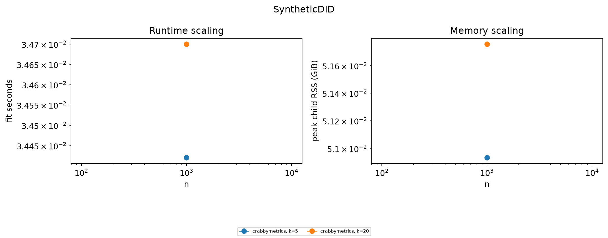
Family and dimensions. panel; k means units; n is periods.

Data-generating process. Low-rank n-period by k-unit panel; treated units are convex mixtures of controls and treatment starts after two thirds of periods.

Fitted specification. SyntheticDID with unit and time penalties fixed at 0.01 and at most 3,000 simplex iterations.

Reference interpretation. R synthdid is the exact external family but is retained as provenance because the package was unavailable in the benchmark environment.

Reference code. r-synthdid

implementation completed cells timeouts RSS kills preflight skips largest completed n largest completed k median fit seconds maximum observed RSS (GiB) median log-log runtime slope k paths with slope
0 crabbymetrics 2 2 0 0 1000 20 0.034561 0.051758 NaN NaN

AugmentedBalancing

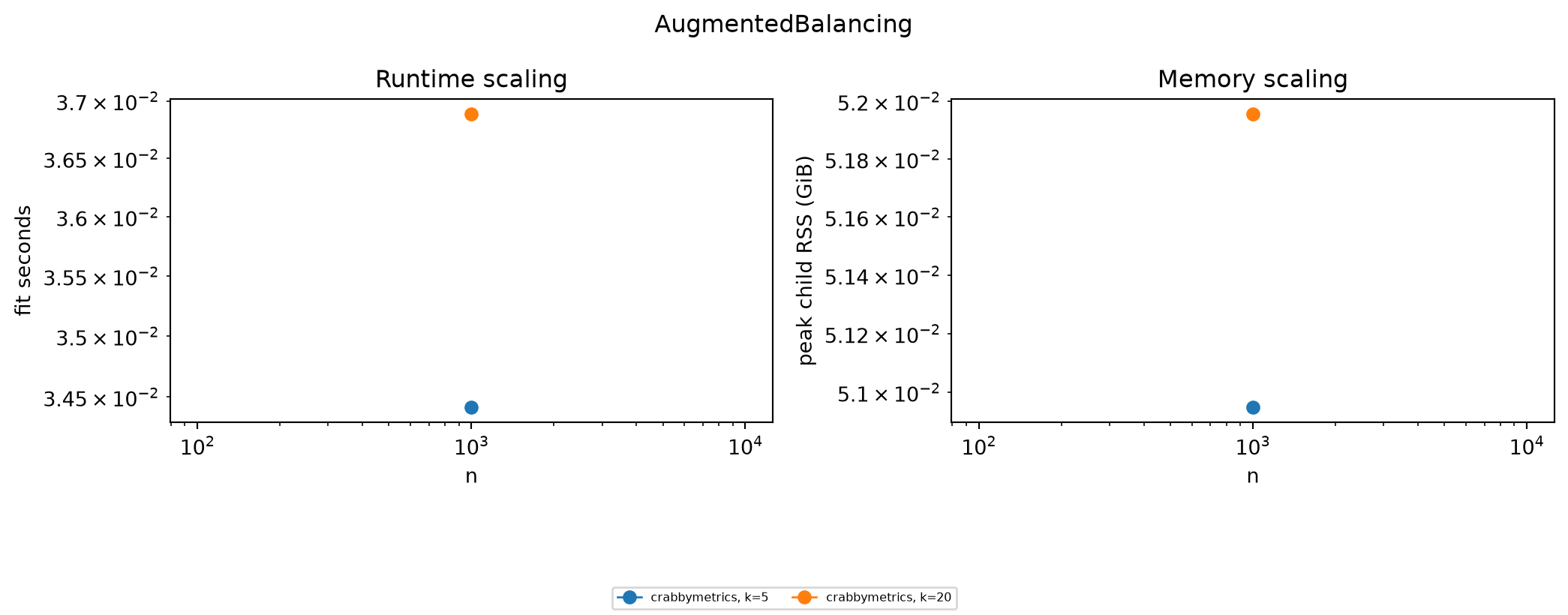
Family and dimensions. panel; k means units; n is periods.

Data-generating process. The same low-rank staggered panel used for SyntheticDID, with no supplied outcome surface so runtime covers raw double balancing.

Fitted specification. Double AugmentedBalancing with unit and time penalties 0.01 and at most 3,000 iterations.

Reference interpretation. R augsynth and the repository’s independent quadprog parity fixture are references; neither is substituted for the exact Crabbymetrics configuration in timing plots.

Reference code. r-augsynth, r-independent-quadprog

implementation completed cells timeouts RSS kills preflight skips largest completed n largest completed k median fit seconds maximum observed RSS (GiB) median log-log runtime slope k paths with slope
0 crabbymetrics 2 2 0 0 1000 20 0.035652 0.051956 NaN NaN

MatrixCompletion

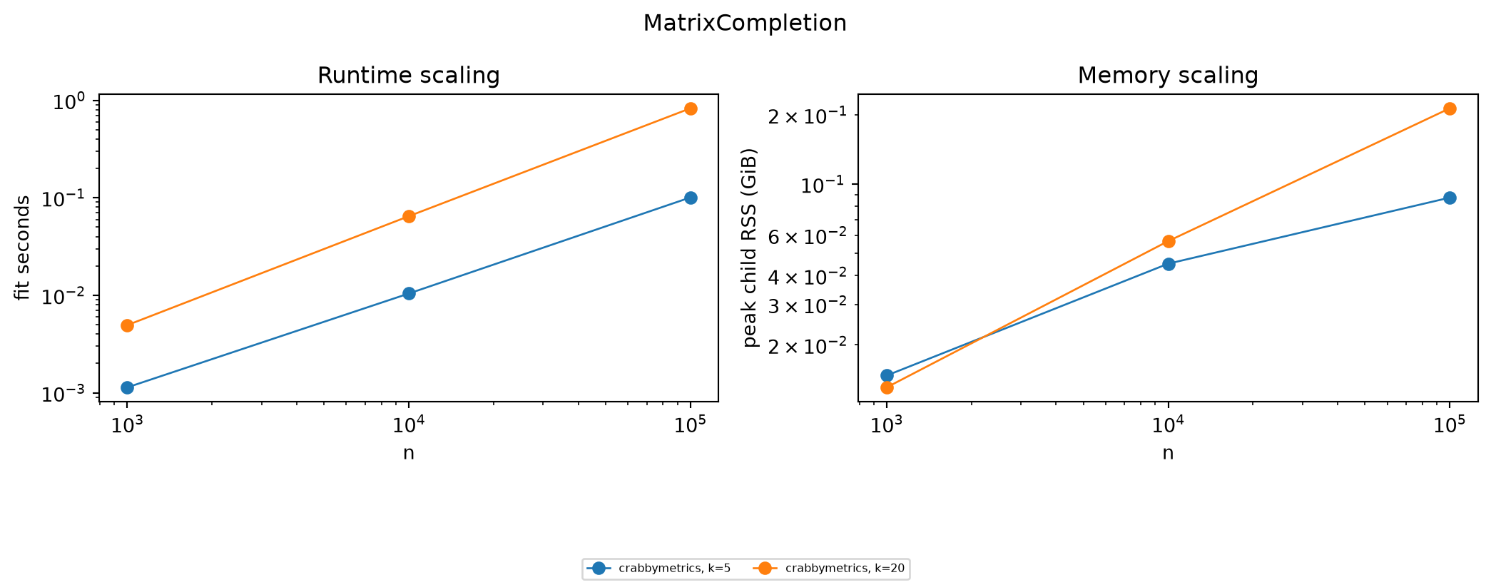
Family and dimensions. panel; k means units; n is periods.

Data-generating process. The low-rank treated panel with n periods and k units.

Fitted specification. MatrixCompletion with at most 50 outer iterations and SVD rank min(6, k-1), retaining unit and time effects.

Reference interpretation. R fect method=mc is the canonical family reference, but its full long-panel interface is not treated as a generic-grid drop-in.

Reference code. r-fect-mc

implementation completed cells timeouts RSS kills preflight skips largest completed n largest completed k median fit seconds maximum observed RSS (GiB) median log-log runtime slope k paths with slope
0 crabbymetrics 6 0 0 0 100000 20 0.037569 0.213562 1.042795 2

InteractiveFixedEffects

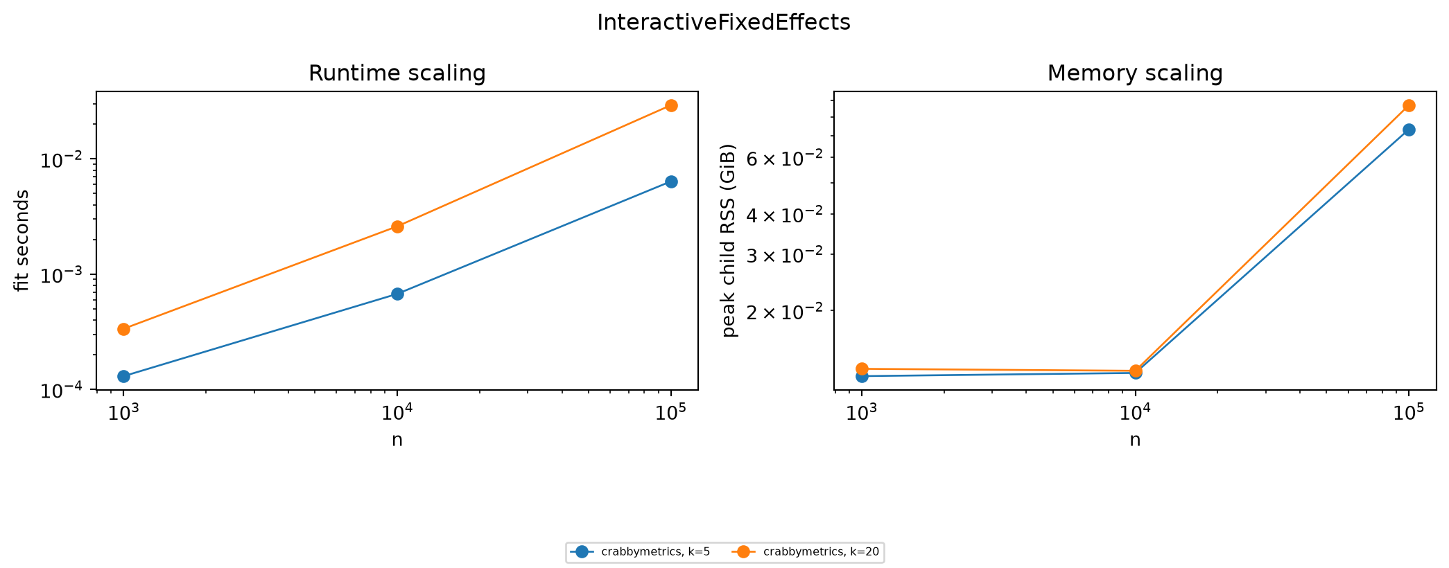
Family and dimensions. panel; k means units; n is periods.

Data-generating process. The untreated low-rank n-period by k-unit outcome matrix from the panel generator.

Fitted specification. InteractiveFixedEffects with rank min(2, k-1) and the default force specification.

Reference interpretation. R fect method=ife and gsynth are canonical family references, not timed substitutes.

Reference code. r-fect-ife, r-gsynth

implementation completed cells timeouts RSS kills preflight skips largest completed n largest completed k median fit seconds maximum observed RSS (GiB) median log-log runtime slope k paths with slope
0 crabbymetrics 6 0 0 0 100000 20 0.001638 0.087006 0.906968 2

BalancingWeights

Family and dimensions. balancing; k means balance functions.

Data-generating process. Gaussian X with the first 80 percent of rows as the source sample and the final 20 percent as the target sample.

Fitted specification. Quadratic BalancingWeights, default box constraints, and at most 100 iterations, balancing k raw covariate means.

Reference interpretation. ebal, WeightIt, and CBPS are provenance because their objectives and constraints are not identical.

Reference code. r-ebal, r-weightit, r-cbps

implementation completed cells timeouts RSS kills preflight skips largest completed n largest completed k median fit seconds maximum observed RSS (GiB) median log-log runtime slope k paths with slope
0 crabbymetrics 6 0 0 0 100000 20 0.001415 0.099442 0.892348 2

MEstimator

Family and dimensions. moments; k means parameters/covariates.

Data-generating process. Gaussian linear outcome with an explicit intercept-augmented n by (k+1) design.

Fitted specification. Generic MEstimator receives a least-squares objective/analytic gradient callback and observation-level score callback, starting at zero for at most 30 iterations.

Reference interpretation. R geex is the callback-framework reference; arbitrary user callbacks prevent a single universal external timing adapter.

Reference code. r-geex

implementation completed cells timeouts RSS kills preflight skips largest completed n largest completed k median fit seconds maximum observed RSS (GiB) median log-log runtime slope k paths with slope
0 crabbymetrics 6 0 0 0 100000 20 0.01288 0.137268 0.901312 2

GMM

Family and dimensions. moments; k means parameters/instruments.

Data-generating process. Exactly identified linear moments X_i(y_i - X_i’ theta) on the intercept-augmented Gaussian linear design.

Fitted specification. Identity-weighted GMM with analytic Jacobian, zero initialization, and at most 30 iterations.

Reference interpretation. R gmm and statsmodels are framework references; their generic callback and covariance work is not forced into a misleading one-size timing row.

Reference code. r-gmm, statsmodels-gmm

implementation completed cells timeouts RSS kills preflight skips largest completed n largest completed k median fit seconds maximum observed RSS (GiB) median log-log runtime slope k paths with slope
0 crabbymetrics 6 0 0 0 100000 20 0.002405 0.070206 0.826685 2

EPLM

Family and dimensions. semiparametric; k means controls.

Data-generating process. Continuous treatment d = 0.25 X beta plus noise and outcome y = 0.8 d + X beta plus noise.

Fitted specification. Crabbymetrics EPLM with its default finite-difference epsilon.

Reference interpretation. DoubleML PLR is related but uses different orthogonalization/cross-fitting, so it is provenance rather than an EPLM speed comparator.

Reference code. doubleml-plr-nearest

implementation completed cells timeouts RSS kills preflight skips largest completed n largest completed k median fit seconds maximum observed RSS (GiB) median log-log runtime slope k paths with slope
0 crabbymetrics 6 0 0 0 100000 20 0.003278 0.108978 0.959074 2

AverageDerivative

Family and dimensions. semiparametric; k means controls.

Data-generating process. The continuous-treatment partially linear design used for EPLM.

Fitted specification. Doubly robust AverageDerivative with default finite-difference epsilon.

Reference interpretation. R np gradient routines are the nearest public reference, not an identical estimator.

Reference code. r-np-gradient-nearest

implementation completed cells timeouts RSS kills preflight skips largest completed n largest completed k median fit seconds maximum observed RSS (GiB) median log-log runtime slope k paths with slope
0 crabbymetrics 6 0 0 0 100000 20 0.015038 0.282532 1.037345 2

PartiallyLinearDML

Family and dimensions. semiparametric; k means controls.

Data-generating process. Continuous treatment d = 0.25 X beta plus noise and outcome y = 0.8 d + X beta plus noise.

Fitted specification. Crabbymetrics PartiallyLinearDML with ridge penalty 0.1 and two folds versus DoubleML PLR with two-fold ridge nuisance learners.

Reference interpretation. Matched partially linear orthogonal-score family with library-specific fold draws and nuisance conventions.

Reference code. doubleml-plr

implementation completed cells timeouts RSS kills preflight skips largest completed n largest completed k median fit seconds maximum observed RSS (GiB) median log-log runtime slope k paths with slope
0 crabbymetrics 6 0 0 0 100000 20 0.006748 0.119156 0.994274 2
1 doubleml-plr 6 0 0 0 100000 20 0.003446 0.319763 0.400633 2

AIPW

Family and dimensions. semiparametric; k means controls.

Data-generating process. Binary treatment obtained by median-splitting 0.25 X beta plus noise; y = 0.8 d + X beta plus noise.

Fitted specification. Crabbymetrics AIPW with ridge penalty 0.1, two folds, and propensity clipping 0.02 versus DoubleML IRM with ridge/logit nuisances and the same clipping threshold.

Reference interpretation. Matched ATE/AIPW family; fold construction and nuisance-standardization details differ.

Reference code. doubleml-irm, econml-drlearner

implementation completed cells timeouts RSS kills preflight skips largest completed n largest completed k median fit seconds maximum observed RSS (GiB) median log-log runtime slope k paths with slope
0 crabbymetrics 6 0 0 0 100000 20 0.007098 0.142609 1.000778 2
1 doubleml-irm 6 0 0 0 100000 20 0.010294 0.330093 0.528996 2

DynamicCovariateBalance

Family and dimensions. dynamic; k means history covariates.

Data-generating process. Approximately n/4 units over four decision periods, k Gaussian history variables per period, logistic treatment driven by the first history coordinate, and a random-walk outcome with additive 0.5 treatment effects.

Fitted specification. DynamicCovariateBalance targets the all-zero four-period path with at most 100 iterations.

Reference interpretation. No exact public Viviano-Bradic implementation was found; the estimator is native-only in the timing grid.

Reference code. native-only-no-public-exact-match

implementation completed cells timeouts RSS kills preflight skips largest completed n largest completed k median fit seconds maximum observed RSS (GiB) median log-log runtime slope k paths with slope
0 crabbymetrics 6 0 0 0 100000 20 0.002132 0.084106 0.688545 2

ParallelTrendsSNMM

Family and dimensions. dynamic; k means history covariates.

Data-generating process. The four-period dynamic-treatment design with a five-column outcome path including baseline.

Fitted specification. ParallelTrendsSNMM with maximum horizon 1, blip treatment mode, two nuisance folds, and fixed seed 1729.

Reference interpretation. gesttools is a nearby SNMM reference but not a parallel-trends SNMM, so it is not timed as equivalent.

Reference code. r-gesttools-nearest

implementation completed cells timeouts RSS kills preflight skips largest completed n largest completed k median fit seconds maximum observed RSS (GiB) median log-log runtime slope k paths with slope
0 crabbymetrics 6 0 0 0 100000 20 0.006411 0.098099 0.990226 2

RegressionBlip

Family and dimensions. dynamic; k means history covariates.

Data-generating process. The four-period dynamic-treatment design with period outcomes aligned to treatment and k history covariates.

Fitted specification. RegressionBlip with one treatment lag and time effects.

Reference interpretation. DTRreg and gesttools are related blip/SNMM references, but neither matches the shipped regression-blip contract exactly.

Reference code. r-dtrreg-nearest, r-gesttools-nearest

implementation completed cells timeouts RSS kills preflight skips largest completed n largest completed k median fit seconds maximum observed RSS (GiB) median log-log runtime slope k paths with slope
0 crabbymetrics 6 0 0 0 100000 20 0.009307 0.142639 1.02754 2

Interpretation

The grid is a systems benchmark, not an accuracy horse race. Fit-only timing is reported; synthetic-data construction happens before the model call but remains inside the child process and therefore contributes to the memory guard. Reference rows test the same shapes and model family, but small differences in defaults, parameterization, convergence criteria, and inference work remain. “Nearest” references in the inventory are literature/code pointers only and never enter the timing plots.

On this host, 26 of 30 native estimators completed at least one \(n=10^6\) cell. The native sample-size frontiers were \(n=10^3\) for synthetic DID and augmented balancing, \(n=10^4\) for Cox PH and Andersen–Gill, and \(n=10^6\) for the other 26 estimators. These maxima collapse across \(k\) and therefore describe reach, not a claim that every dimension completed at that sample size.