An econometric perspective on instrumental variables
Chapter 23 is where the design-based IV story becomes an econometrics workflow: controls, overidentification, and alternative representations of the same parameter.
Show code
from pathlib import Pathimport mathimport matplotlib.pyplot as pltimport numpy as npimport pandas as pdimport crabbymetrics as cmnp.set_printoptions(precision=4, suppress=True)def iv_moments(theta, data): resid = data["y"] - data["x"] @ thetareturn data["z"] * resid[:, None]def iv_jacobian(theta, data):del thetareturn-(data["z"].T @ data["x"]) / data["x"].shape[0]
OLS return to education: 0.0747
OLS HC1 SE: 0.0036
TwoSLS return to education: 0.1571
TwoSLS HC1 SE: 0.0526
Two-step GMM return to education: 0.1552
Two-step GMM SE: 0.0522
GMM J-statistic: 1.2988 with df = 1
The GMM calculation centers and scales nonconstant regressors and instruments: squared experience and binary indicators otherwise have very different scales. The education coefficient and SE are transformed back to log-wage per year of schooling. Scaling changes the finite-sample identity-weighted first step, so this two-step estimate is not required to equal TwoSLS exactly. A tighter tolerance on the raw, poorly scaled system can fail the v0.9 convergence guard even with a small score; a small score alone is not enough.
TwoSLS coefficient: 0.1571
Control-function coefficient on education: 0.1571
4 Anderson-Rubin Grid
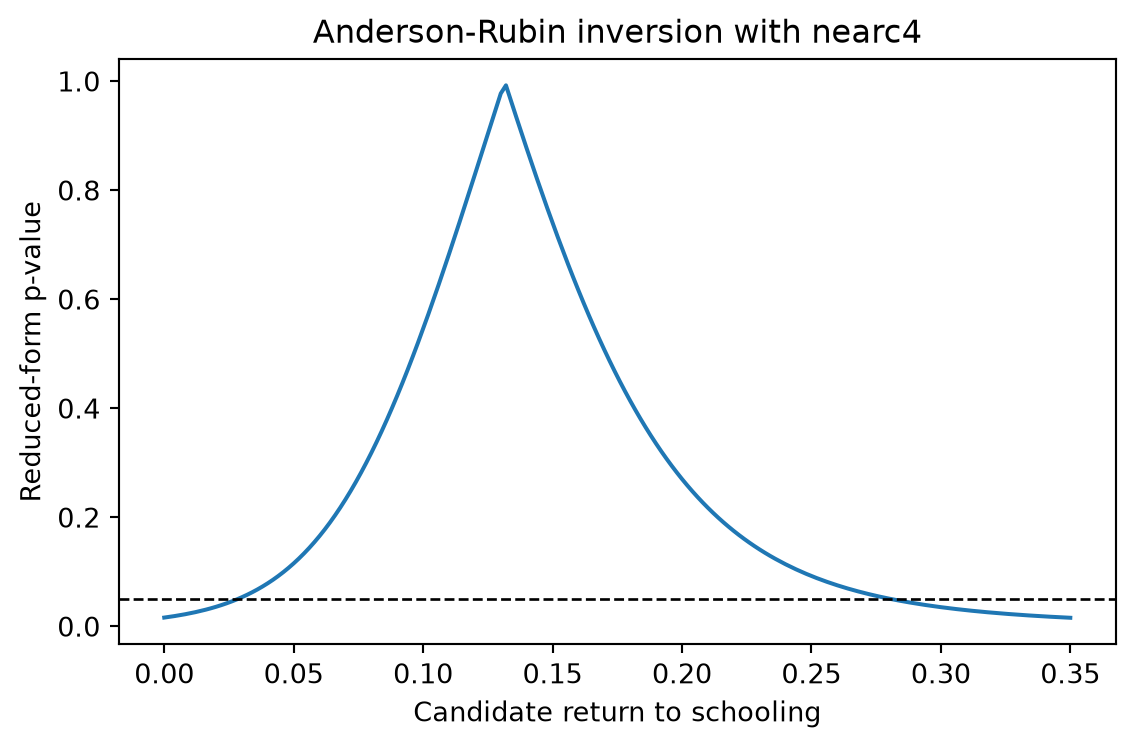
The source R script also inverts a reduced-form test over candidate education returns. For a candidate \(\beta\), regress \(Y - \beta D\) on controls and the excluded instrument. If the excluded instrument is still predictive, that candidate \(\beta\) is inconsistent with the IV moment. This grid uses nearc4, matching the script’s single-instrument Anderson-Rubin calculation.