First Course Ding: Chapter 13

ATT estimation and balancing weights

Chapter 13 shifts attention from the ATE to the ATT. The R script computes outcome-regression, odds-weighted, and doubly robust ATT estimators. This page keeps those formulas and also shows the library-native balancing-weight version, because BalancingWeights directly targets the treated covariate distribution.

Show code

from pathlib import Path

import matplotlib.pyplot as plt
import numpy as np
import pandas as pd

import crabbymetrics as cm

np.set_printoptions(precision=4, suppress=True)


def expit(x):
    return 1.0 / (1.0 + np.exp(-x))

1 NHANES ATT Example

Show code

data = pd.read_csv(Path("../data/ding") / "nhanes_bmi.csv")
y = data["BMI"].to_numpy(dtype=float)
d = data["School_meal"].to_numpy(dtype=np.int32)
x = data[["age", "ChildSex", "black", "mexam", "pir200_plus", "WIC", "Food_Stamp", "AnyIns", "RefAge"]].to_numpy(dtype=float)
x = (x - x.mean(axis=0)) / np.where(x.std(axis=0) > 1e-12, x.std(axis=0), 1.0)

treated = d == 1
control = ~treated

reg0 = cm.OLS()
reg0.fit(x[control], y[control])
y0_hat = reg0.predict(x)
att_reg = float(y[treated].mean() - y0_hat[treated].mean())

reg_all = cm.OLS()
reg_all.fit(np.column_stack([d.astype(float), x]), y)
att_reg0 = float(reg_all.summary()["coef"][0])

logit = cm.Logit(alpha=1.0, max_iterations=300)
logit.fit(x, d)
logit_s = logit.summary()
pscore = expit(logit_s["intercept"] + x @ np.asarray(logit_s["coef"]))
odds = pscore / np.clip(1.0 - pscore, 1e-6, None)
nn = len(y)
nn1 = treated.sum()
res0 = y - y0_hat
att_ht = float(y[treated].mean() - np.mean(odds * (1 - d) * y) * nn / nn1)
odds_w = odds[control] / odds[control].sum()
att_odds = float(y[treated].mean() - np.dot(odds_w, y[control]))
att_dr = float(att_reg - np.mean(odds * (1 - d) * res0) * nn / nn1)

pscore_trunc = np.minimum(pscore, 0.9)
odds_trunc = pscore_trunc / np.clip(1.0 - pscore_trunc, 1e-6, None)
odds_trunc_w = odds_trunc[control] / odds_trunc[control].sum()
att_hajek_trunc = float(y[treated].mean() - np.dot(odds_trunc_w, y[control]))
att_dr_trunc = float(att_reg - np.mean(odds_trunc * (1 - d) * res0) * nn / nn1)

entropy = cm.BalancingWeights(
    objective="entropy",
    solver="auto",
    autoscale=True,
    l2_norm=0.02,
    max_iterations=300,
    tolerance=1e-8,
)
entropy.fit(x[control], x[treated])
entropy_s = entropy.summary()
att_entropy = float(y[treated].mean() - np.dot(np.asarray(entropy_s["weights"]), y[control]))

quad = cm.BalancingWeights(
    objective="quadratic",
    solver="auto",
    autoscale=True,
    l2_norm=0.02,
    max_iterations=300,
    tolerance=1e-8,
)
quad.fit(x[control], x[treated])
quad_s = quad.summary()
att_quad = float(y[treated].mean() - np.dot(np.asarray(quad_s["weights"]), y[control]))

pd.DataFrame(
    {
        "estimate": [
            att_reg0,
            att_reg,
            att_ht,
            att_odds,
            att_dr,
            att_hajek_trunc,
            att_dr_trunc,
            att_entropy,
            att_quad,
        ]
    },
    index=[
        "OLS coefficient on treatment",
        "Outcome-regression ATT",
        "HT odds-weight ATT",
        "Hajek odds-weight ATT",
        "Doubly robust ATT",
        "Hajek ATT, pscore <= 0.9",
        "DR ATT, pscore <= 0.9",
        "Entropy-balancing ATT",
        "Quadratic-balancing ATT",
    ],
)

	estimate
OLS coefficient on treatment	0.048515
Outcome-regression ATT	-0.362396
HT odds-weight ATT	-1.830043
Hajek odds-weight ATT	-0.380848
Doubly robust ATT	-0.204772
Hajek ATT, pscore <= 0.9	-0.191598
DR ATT, pscore <= 0.9	-0.247166
Entropy-balancing ATT	-0.193630
Quadratic-balancing ATT	-0.304733

2 Balance Before And After Weighting

Show code

def standardized_mean_difference(x_treated, x_control, weights=None):
    mt = x_treated.mean(axis=0)
    if weights is None:
        mc = x_control.mean(axis=0)
        vc = x_control.var(axis=0)
    else:
        mc = np.average(x_control, axis=0, weights=weights)
        vc = np.average((x_control - mc) ** 2, axis=0, weights=weights)
    vt = x_treated.var(axis=0)
    scale = np.sqrt(0.5 * (vt + vc))
    scale = np.where(scale > 1e-12, scale, 1.0)
    return (mt - mc) / scale


smd_before = standardized_mean_difference(x[treated], x[control])
smd_entropy = standardized_mean_difference(x[treated], x[control], np.asarray(entropy_s["weights"]))
smd_quad = standardized_mean_difference(x[treated], x[control], np.asarray(quad_s["weights"]))

fig, ax = plt.subplots(figsize=(9, 4))
labels = [f"x{j + 1}" for j in range(x.shape[1])]
xpos = np.arange(len(labels))
width = 0.25
ax.bar(xpos - width, np.abs(smd_before), width=width, label="Unweighted")
ax.bar(xpos, np.abs(smd_entropy), width=width, label="Entropy")
ax.bar(xpos + width, np.abs(smd_quad), width=width, label="Quadratic")
ax.axhline(0.1, color="black", linestyle="--", linewidth=1.0)
ax.set_xticks(xpos)
ax.set_xticklabels(labels)
ax.set_ylabel("Absolute standardized mean difference")
ax.set_title("ATT balance before and after weighting")
ax.legend()
plt.tight_layout()
plt.show()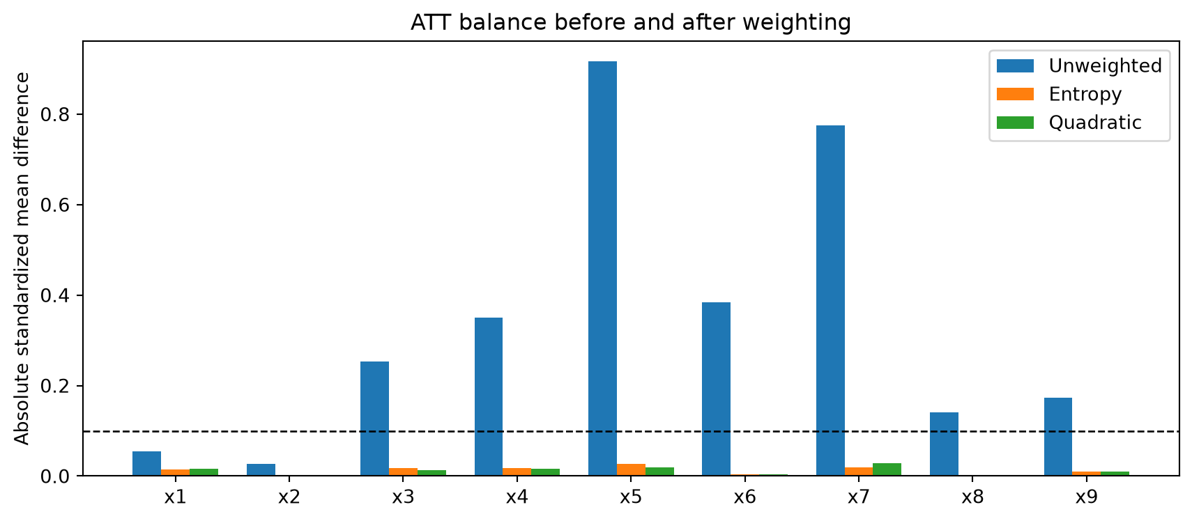

For ATT work, balancing weights are the clean library-native translation of the chapter. They target the treated population directly, which is exactly the estimand shift that Chapter 13 is about.