First Course Ding: Chapter 6

Regression adjustment and rerandomization

Chapter 6 combines two ideas that now look standard:

Lin-style regression adjustment in randomized experiments
rerandomization as a design-stage way to reject badly imbalanced assignments

Show code

from pathlib import Path

import matplotlib.pyplot as plt
import numpy as np
import pandas as pd

import crabbymetrics as cm

np.set_printoptions(precision=4, suppress=True)


data_dir = Path("../data/ding")

1 Regression Adjustment In The STAR Data

Show code

star = pd.read_stata(data_dir / "star.dta")
star = star.query("control == 1 or sfsp == 1").copy()
star["y"] = star["GPA_year1"].fillna(star["GPA_year1"].mean())

y = star["y"].to_numpy(dtype=float)
z = star["sfsp"].to_numpy(dtype=float)
x = star[["female", "gpa0"]].to_numpy(dtype=float)
xc = x - x.mean(axis=0, keepdims=True)

unadjusted = cm.OLS()
unadjusted.fit(z[:, None], y)

lin_design = np.column_stack([z, xc, z[:, None] * xc])
lin = cm.OLS()
lin.fit(lin_design, y)

pd.DataFrame(
    {
        "estimate": [
            unadjusted.summary()["coef"][0],
            lin.summary()["coef"][0],
        ],
        "se_hc1": [
            unadjusted.summary(vcov="hc1")["coef_se"][0],
            lin.summary(vcov="hc1")["coef_se"][0],
        ],
    },
    index=["Unadjusted", "Lin-adjusted"],
)

	estimate	se_hc1
Unadjusted	0.051829	0.077367
Lin-adjusted	0.068166	0.073170

2 A Small Rerandomization Simulation

Show code

rng = np.random.default_rng(6)
n = 250
n1 = n // 2
x = rng.normal(size=(n, 2))
y0 = 0.6 * x[:, 0] - 0.4 * x[:, 1] + rng.normal(scale=0.7, size=n)
tau = 1.0 + 0.25 * x[:, 0]
y1 = y0 + tau


def diff_in_means(y, z):
    treated = z == 1.0
    control = ~treated
    return y[treated].mean() - y[control].mean()


def lin_estimate(y, z, x):
    xc = x - x.mean(axis=0, keepdims=True)
    design = np.column_stack([np.ones(len(y)), z, xc, z[:, None] * xc])
    beta, *_ = np.linalg.lstsq(design, y, rcond=None)
    return beta[1]


def imbalance_score(z, x):
    treated = z == 1.0
    control = ~treated
    diff = x[treated].mean(axis=0) - x[control].mean(axis=0)
    scale = x.std(axis=0, ddof=1)
    return float(np.sum((diff / scale) ** 2))


def draw_assignment(rng, rerandomize=False, threshold=0.08):
    while True:
        z = np.zeros(n)
        z[rng.choice(n, size=n1, replace=False)] = 1.0
        if (not rerandomize) or imbalance_score(z, x) <= threshold:
            return z


mc = 400
records = []
for design_name, rerand in [("Complete randomization", False), ("Rerandomization", True)]:
    for _ in range(mc):
        z_draw = draw_assignment(rng, rerandomize=rerand)
        y_obs = z_draw * y1 + (1.0 - z_draw) * y0
        records.append(
            {
                "design": design_name,
                "diff_in_means": diff_in_means(y_obs, z_draw),
                "lin_adjusted": lin_estimate(y_obs, z_draw, x),
                "imbalance": imbalance_score(z_draw, x),
            }
        )

sim = pd.DataFrame(records)
sim.groupby("design")[["diff_in_means", "lin_adjusted", "imbalance"]].agg(["mean", "std"])

	diff_in_means		lin_adjusted		imbalance
	mean	std	mean	std	mean	std
design
Complete randomization	0.989575	0.133870	0.993991	0.078156	0.032905	0.033030
Rerandomization	0.993091	0.127354	1.003287	0.086698	0.024838	0.020134

Show code

fig, axes = plt.subplots(1, 2, figsize=(10, 4))
for ax, column, title in zip(
    axes,
    ["diff_in_means", "lin_adjusted"],
    ["Unadjusted estimator", "Lin-adjusted estimator"],
):
    for label, df in sim.groupby("design"):
        ax.hist(df[column], bins=35, alpha=0.55, label=label)
    ax.axvline(tau.mean(), color="black", linestyle="--", linewidth=2.0)
    ax.set_title(title)
    ax.legend()
fig.tight_layout()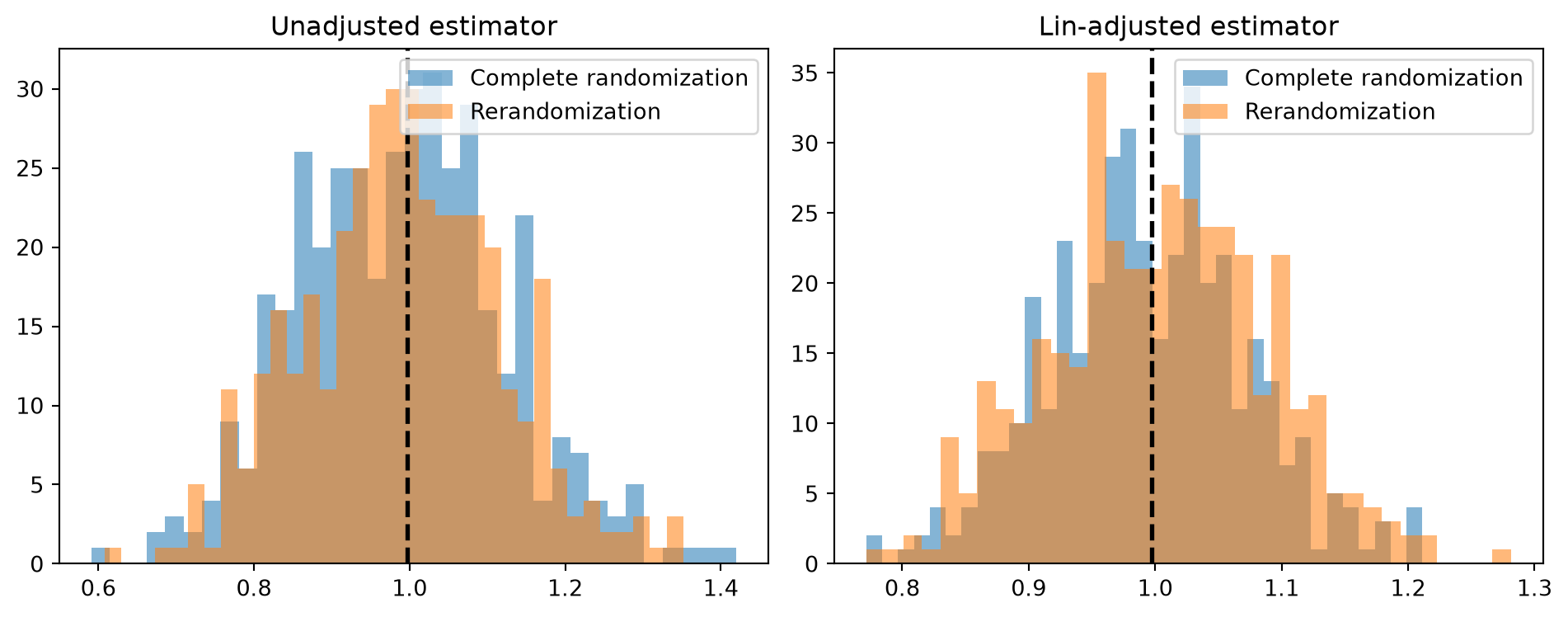

3 Takeaway

Lin adjustment and rerandomization are doing different jobs:

rerandomization changes the assignment rule before outcomes are observed
regression adjustment changes the estimator after the assignment is realized

Both tend to reduce finite-sample noise when the covariates are prognostic.